اللغةintermediateمعالج رسوميات~35 دقيقةColab
قِس قانون التوسّع بنفسك
Fit Your Own Scaling Law
قانون التوسّع نتيجة قياس، وليس ثابتاً
لديك ميزانية حوسبة لم تدرّب عندها أيّ نموذج من قبل، وهي لا تكفي إلا لنموذج واحد. ما الحجم المناسب لهذا النموذج؟ وكم من البيانات يجب أن يقرأ؟ في الأدبيات جواب مشهور: نحو 20 رمزاً تدريبياً لكل معامل. لكنّ هذا الرقم جاء من قياس، على نماذج غيرك وبياناته ومُرمِّزه. في هذا الدفتر تقيس رقمك أنت. تدرّب بضع عشرات من النماذج اللغوية الصغيرة التي تقرأ النص بايتاً بايتاً، ثم توفّق قوانين قوة على أفضلها. بعد ذلك تلتزم بحجم نموذج وبقيمة خسارة، لميزانية أكبر بـ4 مرات من كل ما درّبته. ثم تدرّب عند تلك الميزانية فعلاً، وترى كم ابتعد توقّعك عن الواقع. في هذا الإعداد يخرج القانون على الشكل N ∝ C^0.715. وهذا الأُسّ قريب من أُسّ الورقة الأقدم، لا من أُسّ الورقة الأحدث. ثم إنّ أفضل تقسيم ليس ثابتاً. فهو ينخفض من 166 بايتاً لكل معامل عند أصغر ميزانية، إلى 28 عند الميزانية المحجوزة.
الهدف
أن تتوقّع أفضل حجم للنموذج وخسارته عند ميزانية أكبر بـ4 مرات من أيّ نقطة دخلت في التوفيق. ثم أن تدرّب عند تلك الميزانية وتقيس، فيأتي الفرق بين التوقّع والقياس ضمن حدّ الخطأ المعلن.
يفتح Colab نسخة للقراءة فقط. احفظ نسخة في Drive للاحتفاظ بتعديلاتك.
يحتاج الدفتر إلى لوحة مفاتيح — يُفضَّل فتحه على حاسوب مكتبي.
الأوراق وراء هذه الورشة
في عام 2020 قاس Kaplan وزملاؤه كيف تنخفض النموذج اللغوي كلما زادت المعاملات والبيانات والحوسبة. جاءت كل علاقة من هذه العلاقات على شكل . وكانت نصيحتهم: إذا كبرت الميزانية، فأنفق معظم الزيادة على تكبير النموذج. في عام 2022 أعادت ورقة Chinchilla القياس بعناية أكبر، فوصلت إلى جواب مختلف. الجواب الجديد: كبّر المعاملات ورموز التدريب معاً، بنحو 20 رمزاً لكل معامل.
لم يُستنتج أيٌّ من الجوابين من مبادئ أولى. كلاهما جاء من تدريب نماذج كثيرة، ثم رسم نتائجها، ثم توفيق منحنيات عليها. وهذا يعني أنك تستطيع أن تفعل الشيء نفسه على معالج رسومي واحد. الأرقام التي ستحصل عليها ستكون أرقامك أنت، وهذا بالضبط ما يريد هذا الدفتر أن يريك إياه.
تحقّق من بصمة الشيفرة، ومن أنّ معالجاً رسومياً متّصل. فالشبكة تحتاج إليه.
import azimuth_nb as azimuth

env = azimuth.setup(SLUG, lang=LANG, profile=PROFILE)قِس قانون التوسّع بنفسك
Tesla T4 · 14.6 غ.ب · ذاكرة 12.7 غ.ب · PyTorch 2.11.0+cu130
الملف: free
البيانات:
· tinystories-v2-head.txt — 46,875 KB, verified
· NotoNaskhArabic-Regular.ttf — 242 KB, verified
جاهز · seed=17, corpus_bytes=48000000, val_bytes=1000000, context=128, batch=16, lr=0.006, lr_width=32, init_std=0.02, layers=2, heads=2, width_min=8, width_max=224, width_step=4, budget_min=1000000000000, budget_factor=2, n_budgets=4, ratio_min=3, ratio_max=450, n_ratios=7, min_tokens=2000000, holdout_factor=4
الشيفرة · 115a4e6bdc671638تقرأ النماذج البايتات الخام كما هي. لذلك تتكوّن المفردات من 256 رمزاً فقط، ولا يوجد مُرمِّز نحتاج إلى تدريبه أو إلى الاختلاف حوله. وكل خسارة تُقاس بوحدة نات لكل بايت، على نص لم تتدرّب عليه النماذج أبداً.
أول رقم يستحقّ الانتباه هو خط الأساس الأحادي. وهو خسارة نموذج يتجاهل السياق تماماً، ويتوقّع كل بايت من تكراره العام في النص. كل نموذج مدرَّب يجب أن يتفوّق على هذا الخط بفارق واضح. فإذا لم يتفوّق عليه نموذج ما، فهذا النموذج لم يتعلّم شيئاً. وأيّ منحنى نوفّقه عبر نقطة كهذه هو منحنى يمرّ عبر ضجيج.
يقع خط الأساس قرب 3 نات لكل بايت. احفظ هذا الرقم، فكل نموذج مدرَّب يجب أن ينتهي أدنى منه بكثير.
import math

import numpy as np
import torch


def tr(en, ar):
    """Pick the printed string for the notebook's language."""
    return ar if env.lang == "ar" else en


cfg = env.cfg
device = "cuda" if torch.cuda.is_available() else "cpu"
torch.manual_seed(cfg["seed"])

raw = np.frombuffer(env.assets["tinystories-v2-head.txt"].read_bytes(), dtype=np.uint8)
raw = raw[: int(cfg["corpus_bytes"])]
n_val = int(cfg["val_bytes"])
val_bytes, train_bytes = raw[:n_val], raw[n_val:]

# The zero-skill reference: predict every byte from its overall frequency.
counts = np.bincount(train_bytes, minlength=256).astype(np.float64)
probs = counts[counts > 0] / counts.sum()
unigram_loss = round(float(-(probs * np.log(probs)).sum()), 4)

# Cut the training bytes into non-overlapping windows and shuffle them ONCE.
# Every run reads a prefix of this same order, so no run sees a byte twice and
# all runs at all sizes see the same data in the same sequence.
ctx = int(cfg["context"])
n_chunks = len(train_bytes) // (ctx + 1)
train_chunks = (
    torch.from_numpy(train_bytes[: n_chunks * (ctx + 1)].copy()).view(n_chunks, ctx + 1).to(device)
)
order = torch.randperm(n_chunks, generator=torch.Generator().manual_seed(cfg["seed"])).to(device)
max_train_tokens = n_chunks * ctx

n_val_chunks = len(val_bytes) // (ctx + 1)
val_chunks = (
    torch.from_numpy(val_bytes[: n_val_chunks * (ctx + 1)].copy())
    .view(n_val_chunks, ctx + 1)
    .to(device)
)

print(
    tr(
        f"device {device} · train {len(train_bytes) / 1e6:.1f} MB · val {len(val_bytes) / 1e6:.2f} MB",
        f"الجهاز {device} · بيانات التدريب {len(train_bytes) / 1e6:.1f} ميغابايت · التحقق {len(val_bytes) / 1e6:.2f} ميغابايت",
    )
)
print(
    tr(
        f"unigram baseline: {unigram_loss:.3f} nats/byte",
        f"خط الأساس الأحادي: {unigram_loss:.3f} نات لكل بايت",
    )
)
print(train_bytes[:300].tobytes().decode("utf-8", errors="replace"))الجهاز cuda · بيانات التدريب 47.0 ميغابايت · التحقق 1.00 ميغابايت
خط الأساس الأحادي: 3.086 نات لكل بايت
fixed the mailbox! I made it bigger for more letters." Lily was happy. Now she could send her letter to Max. They both walked home, smiling and laughing.
<|endoftext|>
Once upon a time, there was a bossy giant. He lived in a big house on a hill. All the people in the town were scared of him. One dayقانون التوسّع يقارن بين نماذج بأحجام مختلفة، لذلك نحتاج إلى عائلة كاملة منها. لعائلتنا مفتاح واحد فقط. عدد الطبقات ثابت في كل النماذج، وقيمته في ملف التشغيل هي 2، والذي يتغيّر هو العرض وحده. وبتغيير العرض ينتقل الحجم من بضعة آلاف من إلى أكثر من مليون. وتثبيت العمق يضمن أنّ أيّ نموذجين يختلفان في الحجم، ولا يختلفان في شيء آخر.
بجانب كل نموذج عددان للمعاملات. الأول هو العدد الكلي، كما عدّتها ورقة Chinchilla. والثاني هو العدد بعد حذف جداول التضمين، كما عدّها Kaplan. أما العمود الأخير فيبيّن حصّة جداول التضمين من كل نموذج. نستخدم العدد الكلي الآن، ونعود إلى الفرق بين العددين في أحد التمارين.
انظر إلى العمود الأخير. في أضيق النماذج تشكّل جداول التضمين معظم المعاملات، وفي أعرضها جزءاً صغيراً.
import torch.nn as nn
import torch.nn.functional as F

n_layer, n_head = int(cfg["layers"]), int(cfg["heads"])


class Block(nn.Module):
    def __init__(self, d):
        super().__init__()
        self.ln1 = nn.LayerNorm(d)
        self.qkv = nn.Linear(d, 3 * d)
        self.proj = nn.Linear(d, d)
        self.ln2 = nn.LayerNorm(d)
        self.mlp = nn.Sequential(nn.Linear(d, 4 * d), nn.GELU(), nn.Linear(4 * d, d))

    def forward(self, x):
        b, t, d = x.shape
        q, k, v = self.qkv(self.ln1(x)).split(d, dim=2)
        q, k, v = (z.view(b, t, n_head, d // n_head).transpose(1, 2) for z in (q, k, v))
        y = F.scaled_dot_product_attention(q, k, v, is_causal=True)
        x = x + self.proj(y.transpose(1, 2).reshape(b, t, d))
        return x + self.mlp(self.ln2(x))


class TinyLM(nn.Module):
    """A byte-level GPT. The output layer shares weights with the input embedding."""

    def __init__(self, width, init_std):
        super().__init__()
        self.tok = nn.Embedding(256, width)
        self.pos = nn.Embedding(ctx, width)
        self.blocks = nn.ModuleList(Block(width) for _ in range(n_layer))
        self.ln_f = nn.LayerNorm(width)
        # The token table is also the output layer, so its scale sets the size
        # of the very first predictions. Small values start every run near
        # "all 256 bytes equally likely", which is where an untrained model
        # should start.
        nn.init.normal_(self.tok.weight, std=init_std)
        nn.init.normal_(self.pos.weight, std=init_std)

    def forward(self, idx):
        x = self.tok(idx) + self.pos(torch.arange(idx.shape[1], device=idx.device))
        for blk in self.blocks:
            x = blk(x)
        return self.ln_f(x) @ self.tok.weight.T


def count_params(width):
    """Two bookkeeping conventions for the same network."""
    block = 12 * width * width + 13 * width  # attention + MLP + norms
    embedding = 256 * width + ctx * width  # token + position tables
    non_embedding = n_layer * block + 2 * width  # + the final norm
    return {"total": non_embedding + embedding, "non_embedding": non_embedding}


# One family, one knob. Depth is fixed and only the width changes, so "model
# size" is a single number and no run differs from another in shape.
widths = list(range(cfg["width_min"], cfg["width_max"] + 1, cfg["width_step"]))
sizes = {w: count_params(w) for w in widths}

# The formula must agree with the network itself.
for w in (widths[0], widths[-1]):
    real = sum(p.numel() for p in TinyLM(w, cfg["init_std"]).parameters())
    assert real == sizes[w]["total"], (w, real, sizes[w])

print(
    tr(
        f"{len(widths)} models, {n_layer} layers each, "
        f"from {sizes[widths[0]]['total']:,} to {sizes[widths[-1]]['total']:,} parameters",
        f"{len(widths)} نموذجاً، في كلٍّ منها {n_layer} طبقات، "
        f"من {sizes[widths[0]]['total']:,} إلى {sizes[widths[-1]]['total']:,} معاملاً",
    )
)
print(
    tr(
        " width   params (total)   non-embedding   embedding share",
        " العرض   المعاملات (الكلّ)   دون التضمين   حصّة التضمين",
    )
)
for w in widths[:: max(1, len(widths) // 8)]:
    n = sizes[w]
    share = 1 - n["non_embedding"] / n["total"]
print(f"{w:>6} {n['total']:>14,} {n['non_embedding']:>13,} {share:>14.0%}")55 نموذجاً، في كلٍّ منها 2 طبقات، من 4,832 إلى 1,296,512 معاملاً
العرض المعاملات (الكلّ) دون التضمين حصّة التضمين
8 4,832 1,760 64%
32 37,760 25,472 33%
56 98,336 76,832 22%
80 186,560 155,840 16%
104 302,432 262,496 13%
128 445,952 396,800 11%
152 617,120 558,752 9%
176 815,936 748,352 8%
200 1,042,400 965,600 7%
224 1,296,512 1,210,496 7%تدريب محوّل فيه N معاملاً على D رمزاً يكلّف تقريباً C ≈ 6·N·D من عمليات الفاصلة العائمة. ومصدر الرقم 6: عمليتان لكل معامل ولكل رمز في المرور الأمامي، وأربع عمليات في المرور الخلفي. هذا التقريب هو ما يسمح لنا بالمقايضة بين N وD عند ثابتة.
قانون التوسّع يقارن تشغيلات قصيرة بأخرى طويلة، ونماذج ضيّقة بأخرى عريضة. لذلك يجب أن يعامل المدرِّب الجميع بإنصاف. وفيه ثلاثة تفاصيل وُضعت لهذا الغرض.
الأول: جدول معدّل التعلّم في كل تشغيل يمتدّ على طول ذلك التشغيل نفسه. أشار مؤلفو Chinchilla إلى أنّ استخدام جدول واحد لكل التشغيلات كان من أسباب ميل القانون الأقدم إلى النماذج الكبيرة. فالخسارة التي تُقرأ في منتصف جدول طويل تجعل التدريب القصير يبدو أسوأ من حقيقته.
الثاني: جدول التضمين يبدأ بقيم صغيرة. بذلك يبدأ كل تشغيل من تخمين محايد، ولا يُنفق خطواته الأولى في إصلاح بداية سيئة.
الثالث: النماذج الأعرض تأخذ معدّل تعلّم أصغر. فلو استخدمنا معدّلاً واحداً لكل الأحجام، لتدرّبت النماذج الضيّقة أو العريضة تدريباً سيئاً.
هذه ثلاث قواعد بسيطة، ولم نضبط أيّاً منها لتشغيل بعينه. والقانون الذي ستقيسه يخصّ هذه القواعد بقدر ما يخصّ النماذج. وفي أحد التمارين الأخيرة نكسر القاعدة الثانية عمداً، لنرى أثرها.
تشغيل صغير واحد قبل الشبكة. ويجب أن تكون خسارته أدنى من خط الأساس الأحادي منذ الآن.
import time


def train_run(width, tokens, init_std=None):
    """Train one model on exactly `tokens` fresh tokens; return its validation loss.

    The cosine schedule is stretched to this run's own length. That detail is the
    one the Chinchilla paper singles out: a schedule set for a longer run leaves
    a shorter run undertrained, and the scaling law inherits the error.

    The seed depends only on the width, so the same model starts from the same
    weights at every budget.
    """
    batch = int(cfg["batch"])
    steps = max(1, round(tokens / (batch * ctx)))
    assert steps * batch <= n_chunks, "run would repeat data; lower the budget"
    torch.manual_seed(cfg["seed"] + width)
    model = TinyLM(width, cfg["init_std"] if init_std is None else init_std).to(device)
    # Wider layers take smaller steps: the peak learning rate falls with the
    # square root of the width. With one rate for every size, either the narrow
    # models or the wide ones would be trained badly, and each valley would lean
    # toward whichever side the rate happened to suit.
    peak_lr = cfg["lr"] * math.sqrt(cfg["lr_width"] / width)
    opt = torch.optim.AdamW(model.parameters(), lr=peak_lr, betas=(0.9, 0.95), weight_decay=0.1)
    warmup = max(1, int(0.05 * steps))

    def lr_at(step):
        if step < warmup:
            return (step + 1) / warmup
        progress = (step - warmup) / max(1, steps - warmup)
        return 0.1 + 0.9 * 0.5 * (1 + math.cos(math.pi * progress))

    sched = torch.optim.lr_scheduler.LambdaLR(opt, lr_at)
    model.train()
    for step in range(steps):
        rows = train_chunks[order[step * batch : (step + 1) * batch]].long()
        x, y = rows[:, :-1], rows[:, 1:]
        loss = F.cross_entropy(model(x).view(-1, 256), y.reshape(-1))
        opt.zero_grad(set_to_none=True)
        loss.backward()
        torch.nn.utils.clip_grad_norm_(model.parameters(), 1.0)
        opt.step()
        sched.step()
    return evaluate(model), steps * batch * ctx


@torch.no_grad()
def evaluate(model):
    model.eval()
    total, n = 0.0, 0
    for i in range(0, len(val_chunks), 256):
        rows = val_chunks[i : i + 256].long()
        logits = model(rows[:, :-1])
        total += F.cross_entropy(
            logits.reshape(-1, 256), rows[:, 1:].reshape(-1), reduction="sum"
        ).item()
        n += rows[:, 1:].numel()
    return total / n


# One short run to make sure the loop learns before the grid spends real time.
t0 = time.time()
probe_loss, _ = train_run(widths[len(widths) // 4], int(cfg["min_tokens"]))
probe_loss = round(probe_loss, 4)
print(
    tr(
        f"probe run: loss {probe_loss:.3f} nats/byte (unigram {unigram_loss:.3f}) in {time.time() - t0:.1f}s",
        f"تشغيل تجريبي: الخسارة {probe_loss:.3f} نات لكل بايت (الأحادي {unigram_loss:.3f}) خلال {time.time() - t0:.1f} ث",
    )
)تشغيل تجريبي: الخسارة 1.774 نات لكل بايت (الأحادي 3.086) خلال 17.4 ثهنا قلب الطريقة. اختر ميزانية حوسبة C. ثم درّب عدّة نماذج تنفق كلها C بالضبط: من نموذج كبير يقرأ رموزاً قليلة، إلى نموذج صغير يقرأ رموزاً كثيرة. بعد ذلك ارسم خسائرها مقابل أحجامها. الناتج هو (IsoFLOP)، وأدنى نقطة فيه هي أفضل حجم لتلك الميزانية. وتكرّر ذلك لعدّة ميزانيات.
نختار طرق التقسيم بحسب نسبة الرموز إلى المعاملات، D / N. ونوزّع هذه النسب على مدى واسع عن قصد. فنحن لا نعرف مسبقاً أين يقع أفضل تقسيم. والطريقة لا تنجح إلا إذا وُجدت، في كل ميزانية، تشغيلات أسوأ من أفضل تشغيل على جانبيه كليهما.
كل سطر يمثّل ميزانية واحدة. وكلما كبرت الميزانية، انزاح السطر كله نحو نماذج أكبر.
# Compute budgets, spaced by a constant factor. Within a budget C, each run
# splits the same compute differently: N parameters trained on D = C / (6 N)
# tokens. The splits are chosen by tokens-per-parameter ratio, D / N, over a
# wide range, because we do not know in advance where the best split lies.
budgets = [cfg["budget_min"] * cfg["budget_factor"] ** i for i in range(cfg["n_budgets"])]
ratios = np.geomspace(cfg["ratio_min"], cfg["ratio_max"], cfg["n_ratios"])


def affordable(C, w):
    """A split is allowed only if the run gets at least `min_tokens`, and no
    more tokens than the corpus holds, so no run repeats data."""
    return cfg["min_tokens"] <= C / (6 * sizes[w]["total"]) <= max_train_tokens


def plan_budget(C):
    """The widths to train at budget C: the family member nearest each target ratio."""
    chosen = set()
    for ratio in ratios:
        target = math.sqrt(C / (6 * ratio))
        w = min(widths, key=lambda w: abs(math.log(sizes[w]["total"] / target)))
        if affordable(C, w):
            chosen.add(w)
    return sorted(chosen)


def run_record(C, width, loss, tokens):
    n = sizes[width]
    return {
        "C": C,
        "width": width,
        "N": n["total"],
        "N_ne": n["non_embedding"],
        "D": tokens,
        "loss": loss,
    }


plan = [(C, w) for C in budgets for w in plan_budget(C)]
assert all(sum(C_ == C for C_, _ in plan) >= 3 for C in budgets), "a budget has too few sizes"
planned_tokens = sum(C / (6 * sizes[w]["total"]) for C, w in plan)
print(
    tr(
        f"{len(plan)} runs across {len(budgets)} budgets · {planned_tokens / 1e6:.0f}M tokens in total",
        f"{len(plan)} تشغيلاً على {len(budgets)} ميزانيات · {planned_tokens / 1e6:.0f} مليون رمز إجمالاً",
    )
)
for C in budgets:
    shown = ", ".join(f"{sizes[w]['total'] / 1e3:.0f}k" for C_, w in plan if C_ == C)
print(f" C = {C:.1e} FLOPs → N = {shown}")21 تشغيلاً على 4 ميزانيات · 165 مليون رمز إجمالاً
C = 1.0e+12 FLOPs → N = 18k, 30k, 46k, 65k
C = 2.0e+12 FLOPs → N = 30k, 38k, 65k, 98k, 139k
C = 4.0e+12 FLOPs → N = 38k, 55k, 86k, 139k, 204k, 302k
C = 8.0e+12 FLOPs → N = 55k, 86k, 125k, 187k, 281k, 446kأطول خلية في الدفتر. اقرأ الجدول ميزانيةً ميزانية: كلما كبر N انخفضت الخسارة ثم ارتفعت من جديد. وراقب عمود الخطوات.
runs = []
t_grid = time.time()
for i, (C, w) in enumerate(plan):
    loss, tokens = train_run(w, C / (6 * sizes[w]["total"]))
    runs.append(run_record(C, w, loss, tokens))
    if i == 0 or (i + 1) % 5 == 0 or i + 1 == len(plan):
        done = sum(r["D"] for r in runs) / planned_tokens
        eta = max(0.0, (time.time() - t_grid) / done * (1 - done) / 60)
        print(
            tr(
                f"  {i + 1}/{len(plan)} runs · ~{eta:.0f} min left",
                f"  {i + 1}/{len(plan)} تشغيلاً · بقي نحو {eta:.0f} دقيقة",
            )
        )


def print_runs(rows):
    print(
        tr(
            "   budget C     params N     tokens D    steps     D/N    loss",
            "   الميزانية C   المعاملات N   الرموز D   الخطوات     D/N    الخسارة",
        )
    )
    for r in rows:
        steps = r["D"] // (cfg["batch"] * ctx)
        print(
            f"  {r['C']:.1e}  {r['N']:>10,}  {r['D'] / 1e6:>8.2f}M  {steps:>7,}  {r['D'] / r['N']:>6.0f}  {r['loss']:.4f}"
        )


print()
print_runs(runs)

n_runs = len(runs)
grid_minutes = round((time.time() - t_grid) / 60, 1)
worst_margin = round(min(unigram_loss - r["loss"] for r in runs), 3) 1/21 تشغيلاً · بقي نحو 6 دقيقة
5/21 تشغيلاً · بقي نحو 5 دقيقة
10/21 تشغيلاً · بقي نحو 4 دقيقة
15/21 تشغيلاً · بقي نحو 3 دقيقة
20/21 تشغيلاً · بقي نحو 0 دقيقة
21/21 تشغيلاً · بقي نحو 0 دقيقة
الميزانية C المعاملات N الرموز D الخطوات D/N الخسارة
1.0e+12 17,840 9.34M 4,562 524 1.4915
1.0e+12 30,352 5.49M 2,681 181 1.3980
1.0e+12 45,936 3.63M 1,772 79 1.4365
1.0e+12 64,592 2.58M 1,260 40 1.6986
2.0e+12 30,352 10.98M 5,362 362 1.3216
2.0e+12 37,760 8.83M 4,310 234 1.2852
2.0e+12 64,592 5.16M 2,520 80 1.2537
2.0e+12 98,336 3.39M 1,655 34 1.2700
2.0e+12 138,992 2.40M 1,171 17 1.5905
4.0e+12 37,760 17.66M 8,621 468 1.2221
4.0e+12 54,880 12.15M 5,932 221 1.1801
4.0e+12 86,320 7.72M 3,771 89 1.1193
4.0e+12 138,992 4.80M 2,342 35 1.1427
4.0e+12 203,952 3.27M 1,596 16 1.2178
4.0e+12 302,432 2.20M 1,076 7 1.4549
8.0e+12 54,880 24.30M 11,863 443 1.1301
8.0e+12 86,320 15.45M 7,542 179 1.0668
8.0e+12 124,672 10.69M 5,222 86 1.0331
8.0e+12 186,560 7.15M 3,490 38 1.0380
8.0e+12 281,200 4.74M 2,315 17 1.0896
8.0e+12 445,952 2.99M 1,460 7 1.2783إعداد للرسوم فقط. وفي الدفتر العربي يحمّل أيضاً خطاً يحتوي الحروف العربية.
import matplotlib.pyplot as plt
from matplotlib import font_manager
from matplotlib.ticker import FuncFormatter, LogLocator, NullFormatter

if env.lang == "ar":
    # matplotlib draws Arabic as isolated letters in logical order. Reshape the
    # letters into their joined forms and reorder for display, and use a font
    # that actually contains Arabic glyphs (the default DejaVu does not).
    import arabic_reshaper
    from bidi.algorithm import get_display

    font_path = env.assets["NotoNaskhArabic-Regular.ttf"]
    font_manager.fontManager.addfont(str(font_path))
    arabic_font = font_manager.FontProperties(fname=str(font_path)).get_name()
    # Naskh has no Latin glyphs; DejaVu fills in digits, "C", "N" and symbols.
    plt.rcParams["font.family"] = [arabic_font, "DejaVu Sans"]
    plt.rcParams["mathtext.fontset"] = "dejavusans"
    plt.rcParams["axes.unicode_minus"] = False


def lab(en, ar):
    """A figure label in the notebook's language, ready for matplotlib."""
    if env.lang != "ar":
        return en
    return get_display(arabic_reshaper.reshape(ar))


def log_axis(axis, sizes=False):
    """Log ticks as plain text that renders in either font: 3e12, or 50k for sizes."""
    if sizes:
        axis.set_major_locator(LogLocator(base=10, subs=(1, 2, 5)))
        axis.set_major_formatter(FuncFormatter(lambda v, _: f"{v / 1e3:g}k"))
    else:
        axis.set_major_formatter(
            FuncFormatter(lambda v, _: f"{v:.0e}".replace("e+0", "e").replace("e+", "e"))
        )
    axis.set_minor_formatter(NullFormatter())


BLUE, ORANGE = "#3b5bdb", "#e8590c"
budget_colors = plt.cm.viridis(np.linspace(0.1, 0.85, len(budgets)))
print(tr("figure text ready", "نصوص الرسوم جاهزة"))نصوص الرسوم جاهزةكل لون يمثّل ميزانية واحدة، والنجوم تحدّد قاع كل وادٍ. راقبها وهي تتحرّك نحو اليمين كلما زادت الحوسبة.
def find_optimum(C, group, count="total"):
    """Locate the best model size among runs that all spent the same compute C.

    Take the lowest-loss run and its two neighbours, and pass a parabola in
    log N through those three points; its vertex is the optimum. The optimum
    counts as measured only if the best run has a neighbour on both sides, so
    the minimum is bracketed.

    `count` chooses which parameter count goes on the x-axis. The training runs
    are the same either way; only the bookkeeping changes.
    """
    key = "N" if count == "total" else "N_ne"
    group = sorted(group, key=lambda r: r[key])
    best = int(np.argmin([r["loss"] for r in group]))
    lo = max(0, min(best - 1, len(group) - 3))
    window = group[lo : lo + 3]
    x = np.log([r[key] for r in window])
    y = np.array([r["loss"] for r in window])
    a2, a1, a0 = np.polyfit(x, y, 2)
    curved = bool(a2 > 0)
    x_star = -a1 / (2 * a2) if curved else float("nan")
    interior = bool(0 < best < len(group) - 1 and curved and x.min() < x_star < x.max())
    if not interior:
        # No bracketed minimum: report the best run we actually trained.
        x_star = math.log(group[best][key])
    # Tokens at the optimum: D = C / (6 N_total). Under the non-embedding
    # convention, map N_ne back to N_total across the fitted runs first.
    n_total_opt = math.exp(np.interp(x_star, x, np.log([r["N"] for r in window])))
    d_opt = C / (6 * n_total_opt)
    return {
        "C": C,
        "C_count": 6 * math.exp(x_star) * d_opt,
        "N_opt": math.exp(x_star),
        "D_opt": d_opt,
        "L_opt": float(np.polyval((a2, a1, a0), x_star)) if interior else group[best]["loss"],
        "interior": interior,
        "fit": (a2, a1, a0),
        "group": group,
        "window": (x.min(), x.max()),
    }


def isoflop_optima(runs, count="total"):
    return [find_optimum(C, [r for r in runs if r["C"] == C], count) for C in budgets]


def draw_valley(ax, o, color, label):
    xs = np.array([r["N"] for r in o["group"]])
    ax.scatter(xs, [r["loss"] for r in o["group"]], color=color, s=28, zorder=3)
    grid_x = np.linspace(o["window"][0] - 0.1, o["window"][1] + 0.1, 100)
    ax.plot(np.exp(grid_x), np.polyval(o["fit"], grid_x), color=color, lw=1.4, label=label)
    if o["interior"]:
        ax.scatter(
            [o["N_opt"]],
            [o["L_opt"]],
            marker="*",
            s=170,
            color=color,
            edgecolor="black",
            linewidth=0.6,
            zorder=4,
        )


optima = isoflop_optima(runs)
bracketed_share = round(sum(o["interior"] for o in optima) / len(budgets), 2)

fig, ax = plt.subplots(figsize=(7.5, 4.6))
for o, color in zip(optima, budget_colors):
    draw_valley(ax, o, color, f"C = {o['C']:.0e}")
ax.set_xscale("log")
log_axis(ax.xaxis, sizes=True)
ax.set_xlabel(lab("parameters N (log scale)", "عدد المعاملات N (مقياس لوغاريتمي)"))
ax.set_ylabel(lab("validation loss (nats/byte)", "خسارة التحقق (نات لكل بايت)"))
ax.set_title(
    lab(
        "IsoFLOP curves: same compute, different splits",
        "منحنيات الحوسبة الثابتة: الحوسبة نفسها بتقسيمات مختلفة",
    )
)
ax.legend(fontsize=8, frameon=False)
plt.tight_layout()
plt.show()


def print_optimum(o):
    flag = "" if o["interior"] else tr("  ← not bracketed", "  ← غير محصور")
    print(
        f"C = {o['C']:.1e}:  N_opt ≈ {o['N_opt'] / 1e3:,.0f}k   D_opt ≈ {o['D_opt'] / 1e6:.1f}M   "
        f"D/N ≈ {o['D_opt'] / o['N_opt']:,.0f}   L ≈ {o['L_opt']:.4f}{flag}"
    )


for o in optima:
    print_optimum(o)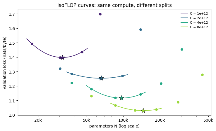
C = 1.0e+12:  N_opt ≈ 32k   D_opt ≈ 5.3M   D/N ≈ 166   L ≈ 1.3975
C = 2.0e+12:  N_opt ≈ 66k   D_opt ≈ 5.1M   D/N ≈ 77   L ≈ 1.2537
C = 4.0e+12:  N_opt ≈ 97k   D_opt ≈ 6.9M   D/N ≈ 71   L ≈ 1.1168
C = 8.0e+12:  N_opt ≈ 146k   D_opt ≈ 9.2M   D/N ≈ 63   L ≈ 1.0298
كل منحنى يشبه وادياً. على يسار القاع نماذج أصغر من اللازم: قرأت بيانات وفيرة، لكن لم تكن لديها سعة كافية للاستفادة منها. وعلى يمين القاع نماذج أكبر مما تحتمله الميزانية: لديها السعة، لكنّ الحوسبة نفدت بعد رموز قليلة. وعند هذا المقياس الصغير، الرموز القليلة تعني خطوات تحسين قليلة. انظر إلى عمود الخطوات في الجدول. التشغيلات على الجدار الأيمن لم تحصل إلا على ما يزيد قليلاً على ألف خطوة. أما النجمة فهي نقطة التوازن بين الحالتين.
لا تُحتسب النجمة إلا إذا وقعت بين تشغيلات حقيقية. يمكن دائماً مدّ القطع المكافئ إلى ما بعد آخر نقطة. لكنّ رأسه هناك تخمين، وليس قياساً. وهذا ما يحرسه فحص الحصر.
ثلاثة توفيقات عبر النجوم: أفضل حجم، وأفضل كمية بيانات، وأفضل خسارة، كلٌّ منها مقابل الحوسبة.
def power_fit(xs, ys):
    """Fit y = k · x^p in log space. Returns (p, k, r2)."""
    lx, ly = np.log(xs), np.log(ys)
    p, logk = np.polyfit(lx, ly, 1)
    resid = ly - (p * lx + logk)
    r2 = 1 - (resid**2).sum() / ((ly - ly.mean()) ** 2).sum()
    return float(p), float(math.exp(logk)), float(r2)


def loss_fit(cs, ls, floor=None):
    """Fit L(C) = E + A · C^(-alpha). Pass `floor` to fix E instead of fitting it.

    E is found by scanning: for each candidate floor, the rest is a straight line
    in log space, so the scan is exact and needs no optimizer.
    """
    cs, ls = np.asarray(cs), np.asarray(ls)
    floors = np.linspace(0.0, ls.min() * 0.995, 400) if floor is None else np.array([floor])
    best = None
    for e in floors:
        slope, logA = np.polyfit(np.log(cs), np.log(ls - e), 1)
        sse = ((e + np.exp(logA) * cs**slope - ls) ** 2).sum()
        if best is None or sse < best[0]:
            best = (sse, float(e), float(math.exp(logA)), float(-slope))
    return best[1], best[2], best[3]  # E, A, alpha


def frontier_points(optima):
    """The optima a frontier may be fitted to, and whether there are enough."""
    good = [o for o in optima if o["interior"]]
    return (good, True) if len(good) >= 3 else (optima, False)


good, enough_interior = frontier_points(optima)
if not enough_interior:
    # An optimum at the edge of the sampled sizes is a guess, not a measurement.
    # Fall back so the cell still runs, but the fit check will fail.
    print(
        tr(
            "⚠ fewer than three budgets have a bracketed optimum; widen the ratio range",
            "⚠ أقلّ من ثلاث ميزانيات لها حجم أمثل محصور بين تجربتين؛ وسّع مدى النِّسب",
        )
    )
C_fit = np.array([o["C"] for o in good])
L_fit = np.array([o["L_opt"] for o in good])
exponent_a, k_N, frontier_r2 = power_fit(C_fit, [o["N_opt"] for o in good])
exponent_b, k_D, _ = power_fit(C_fit, [o["D_opt"] for o in good])
fitted_E, fit_A, alpha_c = loss_fit(C_fit, L_fit)

a_measured, b_measured, E_frontier = round(exponent_a, 3), round(exponent_b, 3), round(fitted_E, 3)
frontier_r2 = round(frontier_r2, 3) if enough_interior else 0.0
ratio_first = round(good[0]["D_opt"] / good[0]["N_opt"])
ratio_last = round(good[-1]["D_opt"] / good[-1]["N_opt"])
tokens_first_m = round(good[0]["D_opt"] / 1e6, 1)
tokens_last_m = round(good[-1]["D_opt"] / 1e6, 1)

print(
    tr(
        f"N_opt ∝ C^{exponent_a:.3f}   (R² {frontier_r2:.3f})\n"
        f"D_opt ∝ C^{exponent_b:.3f}\n"
        f"L_opt(C) = {fitted_E:.3f} + {fit_A:.3g} · C^-{alpha_c:.3f}\n"
        f"tokens per parameter at the best split: {ratio_first} at the smallest fitted budget, "
        f"{ratio_last} at the largest",
        f"N_opt ∝ C^{exponent_a:.3f}   (R² {frontier_r2:.3f})\n"
        f"D_opt ∝ C^{exponent_b:.3f}\n"
        f"L_opt(C) = {fitted_E:.3f} + {fit_A:.3g} · C^-{alpha_c:.3f}\n"
        f"عدد الرموز لكل معامل عند أفضل تقسيم: {ratio_first} عند أصغر ميزانية، "
        f"و{ratio_last} عند أكبرها",
    )
)
print(
    tr(
        "For comparison: Kaplan et al. reported a ≈ 0.73. Chinchilla reported a ≈ 0.50 "
        "and roughly 20 tokens per parameter.",
        "للمقارنة: نشر Kaplan وزملاؤه a ≈ 0.73. ونشرت ورقة Chinchilla a ≈ 0.50، "
        "ونحو 20 رمزاً لكل معامل.",
    )
)N_opt ∝ C^0.715 (R² 0.974)
D_opt ∝ C^0.285
L_opt(C) = 0.637 + 5.58e+03 · C^-0.322
عدد الرموز لكل معامل عند أفضل تقسيم: 166 عند أصغر ميزانية، و63 عند أكبرها
للمقارنة: نشر Kaplan وزملاؤه a ≈ 0.73. ونشرت ورقة Chinchilla a ≈ 0.50، ونحو 20 رمزاً لكل معامل.تقع النجوم قرب خط مستقيم على المقياس اللوغاريتمي. أي أنّ N_opt ∝ C^a، حيث a = 0.715. نشر Kaplan القيمة 0.73، ونشرت Chinchilla القيمة 0.50. قيمتك أقرب إلى قيمة Kaplan. ومعنى ذلك عملياً: حين تتضاعف الميزانية، يذهب معظم الزيادة إلى المعاملات.
التوفيق الثاني يُظهر الوجه الآخر للحقيقة نفسها. عدد الرموز في أفضل تشغيل يكاد لا يتحرّك: D_opt ∝ C^b، حيث b = 0.285. فهو يرتفع من 5.300 مليون رمز عند أصغر ميزانية إلى 9.200 مليون عند أكبرها، مع أنّ الحوسبة تتضاعف عدّة مرات. وعند هذه الميزانيات، بضعة ملايين من الرموز تعني بضعة آلاف من خطوات التحسين. يبدو أنّ التشغيل يحتاج إلى نحو هذا العدد من الخطوات قبل أن يُفيده حجمه. فإذا حصل عليها، صار إنفاق الحوسبة الإضافية على المعاملات أجدى.
إذن عدد الرموز لكل معامل ليس ثابتاً هنا. عند أفضل تقسيم، ينخفض هذا العدد من 166 عند أصغر ميزانية إلى 63 عند أكبرها. أما رقم الـ20 في Chinchilla فكان قياساً لنماذجهم ومُرمِّزهم وبياناتهم، عند ميزانيات أكبر من ميزانياتنا بمراتب كثيرة. لا ينتقل ذلك الرقم إلى إعدادنا، ولا تنتقل أرقامنا إلى إعدادهم. ومن أسباب الفرق وحدة القياس نفسها. فالبايت يحمل معلومات أقلّ بكثير من رمز المُرمِّز، الذي يغطّي عادةً عدّة أحرف.
التوفيق الثالث هو حدّ الخسارة: L_opt(C) = E + A·C^(−α). وهو يُظهر . فكل مضاعفة للحوسبة تُزيل من الخسارة أقلّ مما أزالته المضاعفة التي قبلها. وفي هذا الحدّ أرضية: E = 0.637 نات لكل بايت. هذه الأرضية هي المستوى الذي تقترب منه هذه العائلة من النماذج ولا تتجاوزه، مهما كبرت الميزانية. وهي ، كما تراها هذه النقاط القليلة.
القانون الذي لا يصف إلا النقاط التي وُفِّق عليها هو مجرّد . أما سبب توفيقه أصلاً فهو ، أي اختيار نموذج عند ميزانية لم تجرّبها بعد. لذلك تلتزم الخلية التالية، كتابةً، بحجم نموذج وبقيمة خسارة، لميزانية أكبر بـ4 مرات من أيّ نقطة في التوفيق. وبعدها فقط تبدأ الخلية التي تليها التدريب عند تلك الميزانية.
لا تدريب في هذه الخلية. سجّل الرقمين المتوقَّعين قبل أن تشغّل الخلية التالية.
# Commit to two numbers BEFORE training: the budget is beyond every fitted point.
C_holdout = budgets[-1] * cfg["holdout_factor"]
N_pred = k_N * C_holdout**exponent_a
L_pred = fitted_E + fit_A * C_holdout ** (-alpha_c)

# The model we would actually build: the family member nearest the predicted size.
holdout_widths = plan_budget(C_holdout)
committed_width = min(
    (w for w in widths if affordable(C_holdout, w)),
    key=lambda w: abs(math.log(sizes[w]["total"] / N_pred)),
)
holdout_widths = sorted({*holdout_widths, committed_width})

predicted_size_k = round(N_pred / 1e3)
predicted_loss = round(L_pred, 4)
committed_params = sizes[committed_width]["total"]
committed_tokens_m = round(C_holdout / (6 * committed_params) / 1e6, 1)

print(
    tr(
        f"held-out budget {C_holdout:.1e} FLOPs ({cfg['holdout_factor']}× the largest fitted budget)\n"
        f"predicted best size  N ≈ {predicted_size_k:,}k → we commit to width {committed_width}: "
        f"{committed_params:,} params on {committed_tokens_m:.1f}M tokens\n"
        f"predicted best loss  {predicted_loss:.4f} nats/byte",
        f"الميزانية المحجوزة {C_holdout:.1e} FLOPs (أي {cfg['holdout_factor']} أضعاف أكبر ميزانية في التوفيق)\n"
        f"أفضل حجم متوقَّع  N ≈ {predicted_size_k:,}k ← نلتزم بالعرض {committed_width}: "
        f"{committed_params:,} معاملاً على {committed_tokens_m:.1f} مليون رمز\n"
        f"أفضل خسارة متوقَّعة  {predicted_loss:.4f} نات لكل بايت",
    )
)الميزانية المحجوزة 3.2e+13 FLOPs (أي 4 أضعاف أكبر ميزانية في التوفيق)
أفضل حجم متوقَّع N ≈ 418k ← نلتزم بالعرض 124: 420,112 معاملاً على 12.7 مليون رمز
أفضل خسارة متوقَّعة 0.8865 نات لكل بايتاللوحة اليسرى هي وادي الميزانية الجديدة نفسها. والخطّان الأزرقان المستقيمان هما الرقمان اللذان التزمتَ بهما. انظر كم يقترب قاع الوادي من كلٍّ منهما.
# Train the committed model AND its neighbours at the held-out budget, so the
# budget gets a valley of its own. That is what lets us say whether a miss came
# from choosing the wrong size or from the loss curve itself.
t0 = time.time()
holdout_runs = []
for w in holdout_widths:
    loss, tokens = train_run(w, C_holdout / (6 * sizes[w]["total"]))
    holdout_runs.append(run_record(C_holdout, w, loss, tokens))
holdout_minutes = round((time.time() - t0) / 60, 1)
peak_vram_gb = 0.0
if device == "cuda":
    peak_vram_gb = round(torch.cuda.max_memory_allocated() / 1e9, 2)

print_runs(holdout_runs)
held = find_optimum(C_holdout, holdout_runs)
print()
print_optimum(held)

committed_loss = round(next(r["loss"] for r in holdout_runs if r["width"] == committed_width), 4)
best_holdout_loss = round(min(r["loss"] for r in holdout_runs), 4)
measured_size_k = round(held["N_opt"] / 1e3)
holdout_bracketed = held["interior"]
holdout_ratio = round(held["D_opt"] / held["N_opt"])

# Split the miss in two. `size_regret` is what choosing our size cost, compared
# with the best size we tried. `prediction_error_pct` is how far the predicted
# frontier sits from the best loss this budget actually reached.
size_regret = round(committed_loss - best_holdout_loss, 4)
signed_error_pct = round(100 * (L_pred - best_holdout_loss) / best_holdout_loss, 2)
prediction_error_pct = abs(signed_error_pct)
size_ratio = round(N_pred / held["N_opt"], 2)

print(
    tr(
        f"\nsize:  predicted {predicted_size_k:,}k   measured {measured_size_k:,}k   "
        f"(predicted / measured = {size_ratio:.2f})\n"
        f"loss:  predicted {predicted_loss:.4f}   best measured {best_holdout_loss:.4f}   "
        f"(error {signed_error_pct:+.2f}%)\n"
        f"cost of our size choice: {size_regret:.4f} nats/byte   ({holdout_minutes:.1f} min)",
        f"\nالحجم:  المتوقَّع {predicted_size_k:,}k   المقيس {measured_size_k:,}k   "
        f"(المتوقَّع / المقيس = {size_ratio:.2f})\n"
        f"الخسارة:  المتوقَّعة {predicted_loss:.4f}   أفضل خسارة مقيسة {best_holdout_loss:.4f}   "
        f"(الخطأ {signed_error_pct:+.2f}%)\n"
        f"كلفة اختيارنا للحجم: {size_regret:.4f} نات لكل بايت   ({holdout_minutes:.1f} دقيقة)",
    )
)
if device == "cuda":
    print(
        tr(
            f"peak GPU memory {peak_vram_gb:.2f} GB",
            f"ذروة ذاكرة المعالج الرسومي {peak_vram_gb:.2f} غيغابايت",
        )
    )

fig, (ax0, ax1, ax2) = plt.subplots(1, 3, figsize=(13, 4))
cs = np.geomspace(C_fit.min() / 1.5, C_holdout * 1.5, 100)

draw_valley(ax0, held, ORANGE, lab("held-out budget", "الميزانية المحجوزة"))
ax0.axvline(N_pred, color=BLUE, lw=1.2, ls="--", label=lab("predicted size", "الحجم المتوقَّع"))
ax0.axhline(L_pred, color=BLUE, lw=1.2, ls=":", label=lab("predicted loss", "الخسارة المتوقَّعة"))
ax0.set_xscale("log")
log_axis(ax0.xaxis, sizes=True)
ax0.set_xlabel(lab("parameters N", "عدد المعاملات N"))
ax0.set_ylabel(lab("loss (nats/byte)", "الخسارة (نات لكل بايت)"))
ax0.legend(fontsize=8, frameon=False)

ax1.scatter(
    C_fit,
    [o["N_opt"] for o in good],
    color=BLUE,
    zorder=3,
    label=lab("fitted optima", "أفضل الأحجام في التوفيق"),
)
ax1.plot(cs, k_N * cs**exponent_a, color=BLUE, lw=1.2, ls="--", label=f"N ∝ C^{exponent_a:.2f}")
ax1.scatter(
    [C_holdout],
    [held["N_opt"]],
    marker="D",
    color=ORANGE,
    zorder=4,
    label=lab("measured", "المقيس"),
)
ax1.set_xscale("log")
ax1.set_yscale("log")
log_axis(ax1.xaxis)
log_axis(ax1.yaxis, sizes=True)
ax1.set_xlabel(lab("compute C (FLOPs)", "الحوسبة C بوحدات FLOPs"))
ax1.set_ylabel(lab("best size N", "أفضل حجم N"))
ax1.legend(fontsize=8, frameon=False)

ax2.scatter(C_fit, L_fit, color=BLUE, zorder=3, label=lab("fitted optima", "نقاط التوفيق"))
ax2.plot(
    cs,
    fitted_E + fit_A * cs ** (-alpha_c),
    color=BLUE,
    lw=1.2,
    ls="--",
    label=lab("extrapolated frontier", "الحدّ المُستقرَأ"),
)
ax2.scatter(
    [C_holdout],
    [best_holdout_loss],
    marker="D",
    color=ORANGE,
    zorder=4,
    label=lab("measured", "المقيس"),
)
ax2.set_xscale("log")
log_axis(ax2.xaxis)
ax2.set_ylim(bottom=0)
ax2.set_xlabel(lab("compute C (FLOPs)", "الحوسبة C بوحدات FLOPs"))
ax2.set_ylabel(lab("best loss (nats/byte)", "أفضل خسارة (نات لكل بايت)"))
ax2.legend(fontsize=8, frameon=False)
fig.suptitle(
    lab(
        "Fitted on small budgets, tested on a larger one",
        "توفيق على ميزانيات صغيرة، واختبار على ميزانية أكبر",
    )
)
plt.tight_layout()
plt.show() الميزانية C المعاملات N الرموز D الخطوات D/N الخسارة
3.2e+13 169,936 31.38M 15,324 185 0.9371
3.2e+13 260,736 20.46M 9,988 78 0.9093
3.2e+13 370,736 14.39M 7,024 39 0.9055
3.2e+13 420,112 12.70M 6,199 30 0.9012
3.2e+13 586,672 9.09M 4,439 15 0.9173
3.2e+13 888,352 6.00M 2,931 7 0.9642
3.2e+13 1,296,512 4.11M 2,009 3 1.0303
C = 3.2e+13: N_opt ≈ 434k D_opt ≈ 12.3M D/N ≈ 28 L ≈ 0.9010
الحجم: المتوقَّع 418k المقيس 434k (المتوقَّع / المقيس = 0.96)
الخسارة: المتوقَّعة 0.8865 أفضل خسارة مقيسة 0.9012 (الخطأ -1.63%)
كلفة اختيارنا للحجم: 0.0000 نات لكل بايت (4.3 دقيقة)
ذروة ذاكرة المعالج الرسومي 0.56 غيغابايت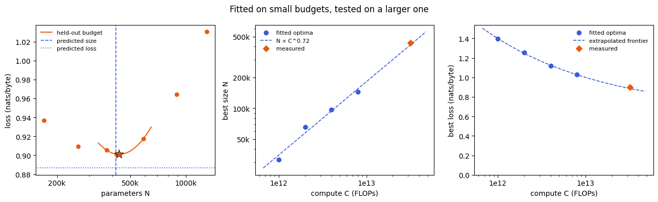
نبدأ بالحجم. توقّع التوفيق أن يكون أفضل حجم قرب 418 ألف معامل. أما قاع وادي الميزانية المحجوزة فيقع قرب 434 ألف. أي أنّ الحجم المتوقَّع يساوي الحجم الأمثل المقيس مضروباً في 0.960. النموذج الذي التزمنا به سجّل خسارة 0.901. وأفضل نموذج درّبناه عند هذه الميزانية سجّل 0.901. الفرق بينهما هو 0 نات لكل بايت، وهذه هي كلفة اختيارنا للحجم.
انظر إلى اللوحة اليسرى لترى لماذا تبقى هذه الكلفة صغيرة. الوادي عريض، ويكاد يكون مستوياً قرب قاعه. لذلك لا يخسر الحجم المنحرف قليلاً عن الأمثل إلا القليل. ولهذا السبب نفسه تنفع القواعد التقريبية للنسبة، حتى حين لا تكون دقيقة.
ننتقل إلى الخسارة. توقّع التوفيق 0.886 نات لكل بايت. وأفضل خسارة مقيسة هي 0.901، أي أنّ الخطأ -1.630%. والإشارة السالبة تعني أنّ التوقّع كان متفائلاً.
هذا هو المنطق نفسه الذي حُدّد به حجم Chinchilla قبل تدريبها، لكن على مقياس أصغر بكثير. تدرّب نماذج صغيرة، ثم تجد قاع كل وادٍ، ثم توفّق الحدّ الأمثل، ثم تستقرئ خارجه. وفي النهاية تفحص هذا الاستقراء عند ميزانية لم تدخل في التوفيق.
الطريقة الثالثة في Chinchilla تستخدم كل التشغيلات معاً، لا النجوم وحدها. فهي توفّق سطحاً واحداً: L(N, D) = E + A/N^α + B/D^β. ثم تقرأ منه أُسّ التوزيع: a = β / (α + β). إذا كانت الطريقتان تصفان الواقع نفسه، فيجب أن تتقاربا. وفي الورقة تقاربتا فعلاً: 0.49 بطريقة الحوسبة الثابتة، و0.46 من السطح. والسطح يعطي أيضاً توقّعه الخاص للميزانية المحجوزة. لذلك نستطيع أن نقيّمه بالطريقة نفسها.
قارن الأُسّين أولاً، ثم قارن توقّعَي الطريقتين للميزانية المحجوزة.
# Chinchilla's third approach: fit one surface L(N, D) = E + A/N^alpha + B/D^beta
# to every fitted run at once, then read the allocation exponent off it.
def fit_surface(rows):
    """Scan the two exponents; solve E, A and B exactly for each pair.

    For fixed alpha and beta the surface is linear in E, A and B, so those three
    come from least squares (on relative error, kept non-negative). Scanning the
    exponents on a grid then finds the best pair with no optimizer to mislead us.
    """
    N = np.array([r["N"] for r in rows], dtype=float)
    D = np.array([r["D"] for r in rows], dtype=float)
    L = np.array([r["loss"] for r in rows])
    ones = np.ones_like(L)
    best = None
    for alpha in np.arange(0.05, 3.0001, 0.025):
        for beta in np.arange(0.05, 3.0001, 0.025):
            X = np.stack([ones, N**-alpha, D**-beta], axis=1) / L[:, None]
            # Drop a term whenever the unconstrained solve would make it negative.
            for cols in ([0, 1, 2], [1, 2], [0, 1], [0, 2]):
                coef = np.linalg.lstsq(X[:, cols], ones, rcond=None)[0]
                if (coef >= 0).all():
                    sse = ((X[:, cols] @ coef - 1) ** 2).sum()
                    if best is None or sse < best[0]:
                        full = np.zeros(3)
                        full[cols] = coef
                        best = (sse, float(alpha), float(beta), full)
                    break
    sse, alpha, beta, (E, A, B) = best
    return {"E": float(E), "A": float(A), "B": float(B), "alpha": alpha, "beta": beta}


def surface_loss(s, N, D):
    return s["E"] + s["A"] / N ** s["alpha"] + s["B"] / D ** s["beta"]


surface = fit_surface(runs)
param_exponent_a = round(surface["beta"] / (surface["alpha"] + surface["beta"]), 3)
param_E = round(surface["E"], 3)

# The surface makes its own prediction for the held-out budget: walk along
# D = C / (6 N) and take the lowest point.
n_grid = np.geomspace(sizes[widths[0]]["total"], sizes[widths[-1]]["total"], 400)
along = surface_loss(surface, n_grid, C_holdout / (6 * n_grid))
surface_size_k = round(float(n_grid[along.argmin()]) / 1e3)
surface_pred = round(float(along.min()), 4)
surface_error_pct = round(100 * (surface_pred - best_holdout_loss) / best_holdout_loss, 2)

print(
    tr(
        f"L(N, D) = {surface['E']:.3f} + {surface['A']:.3g}/N^{surface['alpha']:.3f} "
        f"+ {surface['B']:.3g}/D^{surface['beta']:.3f}\n"
        f"allocation exponent: surface a = β/(α+β) = {param_exponent_a:.3f}"
        f"   ·   IsoFLOP a = {exponent_a:.3f}\n"
        f"irreducible loss E:  surface {param_E:.3f}   ·   frontier {fitted_E:.3f}\n"
        f"held-out budget:     surface predicts N ≈ {surface_size_k:,}k, loss {surface_pred:.4f}"
        f" (error {surface_error_pct:+.2f}%)\n"
        f"                     frontier predicted N ≈ {predicted_size_k:,}k, loss {predicted_loss:.4f}"
        f" (error {signed_error_pct:+.2f}%)\n"
        f"                     measured N ≈ {measured_size_k:,}k, loss {best_holdout_loss:.4f}",
        f"L(N, D) = {surface['E']:.3f} + {surface['A']:.3g}/N^{surface['alpha']:.3f} "
        f"+ {surface['B']:.3g}/D^{surface['beta']:.3f}\n"
        f"أُسّ التوزيع: من السطح a = β/(α+β) = {param_exponent_a:.3f}"
        f"   ·   بطريقة الحوسبة الثابتة a = {exponent_a:.3f}\n"
        f"الخسارة غير القابلة للاختزال E:  من السطح {param_E:.3f}   ·   من الحدّ {fitted_E:.3f}\n"
        f"الميزانية المحجوزة:  يتوقّع السطح N ≈ {surface_size_k:,}k، وخسارة {surface_pred:.4f}"
        f" (الخطأ {surface_error_pct:+.2f}%)\n"
        f"                     وتوقّع الحدّ N ≈ {predicted_size_k:,}k، وخسارة {predicted_loss:.4f}"
        f" (الخطأ {signed_error_pct:+.2f}%)\n"
        f"                     والمقيس N ≈ {measured_size_k:,}k، وخسارة {best_holdout_loss:.4f}",
    )
)L(N, D) = 0.689 + 78.1/N^0.475 + 1.88e+10/D^1.650
أُسّ التوزيع: من السطح a = β/(α+β) = 0.776 · بطريقة الحوسبة الثابتة a = 0.715
الخسارة غير القابلة للاختزال E: من السطح 0.689 · من الحدّ 0.637
الميزانية المحجوزة: يتوقّع السطح N ≈ 486k، وخسارة 0.8894 (الخطأ -1.31%)
وتوقّع الحدّ N ≈ 418k، وخسارة 0.8865 (الخطأ -1.63%)
والمقيس N ≈ 434k، وخسارة 0.9012يعطي السطح a = 0.776 وأرضيةً E = 0.689. وأعطت طريقة الحوسبة الثابتة a = 0.715 وE = 0.637. وللميزانية المحجوزة، توقّع السطح أن يكون أفضل حجم 486 ألف معامل، وأن تكون الخسارة 0.889. أي أنّ خطأه -1.310%.
الطريقتان تقرآن التشغيلات نفسها. لذلك لا يمكن أن يكون الفرق بينهما ضجيجاً في التدريب. مصدر الفرق هو ما تفترضه كل طريقة. السطح يفترض أنّ صيغة واحدة تصحّ في كل التشغيلات، ومنها التشغيلات الواقعة على الجدار الأيمن الحادّ لكل وادٍ. أما طريقة الحوسبة الثابتة فتنظر فقط إلى التشغيلات الثلاثة المحيطة بكل قاع، ولا تفترض شيئاً عن البقية.
وهنا تتّفق الطريقتان في النقاط الأساسية. كلتاهما تعطي أُسّاً أعلى بوضوح من 0.5. وكلتاهما تضع الأرضية عند مستوى متقارب. وكلتاهما تتوقّع للميزانية المحجوزة خسارة قريبة من المقيسة. وحين تصل طريقتان مختلفتا الافتراضات إلى الجواب نفسه، يستحقّ هذا الجواب ثقة أكبر مما يستحقّه أيّ توفيق منفرد.
تمرين
لا يوجد نموذج يتوقّع النص توقّعاً تامّاً. لذلك للحدّ الحقيقي أرضية، وهي الخسارة غير القابلة للاختزال. وقد اضطُرّ التوفيق إلى تقدير هذه الأرضية من بضع نقاط فقط. هذه الخلية تثبّت الأرضية يدوياً، ثم تعيد توفيق بقية المنحنى. وهي تبدأ من الصفر، أي من قانون قوة خالص يستمرّ في الهبوط بلا نهاية. قبل أن تشغّلها، توقّع: هل سيضع هذا القانون خسارة الميزانية المحجوزة أعلى أم أدنى مما وضعها التوفيق ذو الأرضية؟ بعد ذلك ارفع E_FLOOR على خطوات. وراقب رقمين: مدى مطابقة المنحنى لنقاط التوفيق، ومدى قربه من القياس عند الميزانية المحجوزة.
# YOUR TURN — the floor you cannot see.
#
# No model predicts text perfectly, so the true loss curve has a floor E > 0.
# The fit above had to guess E from a handful of points. This cell fixes the
# floor by hand and refits the rest. It starts at zero: a pure power law, which
# keeps falling forever. Before you run it, guess: will that place the held-out
# loss higher or lower than the fit with a floor did? Then raise E_FLOOR in
# steps, and watch two numbers: how well the curve still fits the points it was
# fitted to, and how close it lands at the held-out budget.
E_FLOOR = 0.0

_, A_try, alpha_try = loss_fit(C_fit, L_fit, floor=E_FLOOR)
floor_pred = round(E_FLOOR + A_try * C_holdout ** (-alpha_try), 4)
floor_error_pct = round(100 * (floor_pred - best_holdout_loss) / best_holdout_loss, 2)


def worst_fit_error(E, A, alpha):
    """Largest relative error of a frontier curve on the points it was fitted to."""
    return round(100 * float(np.abs((E + A * C_fit ** (-alpha)) / L_fit - 1).max()), 2)


fitted_in_range_pct = worst_fit_error(fitted_E, fit_A, alpha_c)
in_range_error_pct = worst_fit_error(E_FLOOR, A_try, alpha_try)
print(
    tr(
        f"fitted floor E = {fitted_E:.3f}:  on the fitted points, off by at most {fitted_in_range_pct:.2f}%\n"
        f"    held-out prediction {predicted_loss:.4f}  → error {signed_error_pct:+.2f}%\n"
        f"floor fixed at {E_FLOOR}:  on the fitted points, off by at most {in_range_error_pct:.2f}%\n"
        f"    held-out prediction {floor_pred:.4f}  → error {floor_error_pct:+.2f}%",
        f"الأرضية المُوفَّقة E = {fitted_E:.3f}:  أكبر خطأ على نقاط التوفيق {fitted_in_range_pct:.2f}%\n"
        f"    التوقّع للميزانية المحجوزة {predicted_loss:.4f}  ← الخطأ {signed_error_pct:+.2f}%\n"
        f"الأرضية مثبّتة عند {E_FLOOR}:  أكبر خطأ على نقاط التوفيق {in_range_error_pct:.2f}%\n"
        f"    التوقّع للميزانية المحجوزة {floor_pred:.4f}  ← الخطأ {floor_error_pct:+.2f}%",
    )
)يتوفّر تلميح في الدفتر — env.hint(1)
تمرين
تعيد هذه الخلية توفيق الحدّ الأمثل باستخدام عدد المعاملات دون جداول التضمين. لا يُعاد تدريب أيّ شيء، والذي يتغيّر هو الرقم المكتوب بجانب كل نموذج فقط. قبل أن تشغّلها، خمّن: هل يرتفع الأُسّ a أم ينخفض؟ ثم قارنه بالقيمة التي نشرها Kaplan، أي 0.73، وبقيمة Chinchilla، أي 0.50.
# YOUR TURN — the bookkeeping.
#
# Kaplan et al. counted parameters WITHOUT the embedding tables; Chinchilla
# counted all of them. This cell refits the frontier with the Kaplan count,
# from the very same training runs. Nothing is retrained. Only the number you
# write next to each model changes. Set COUNT = "total" to get the original back.
COUNT = "non_embedding"

recount, _ = frontier_points(isoflop_optima(runs, count=COUNT))
count_exponent_a, _, count_r2 = power_fit(
    [o["C_count"] for o in recount], [o["N_opt"] for o in recount]
)
count_exponent_a = round(count_exponent_a, 3)
count_ratio_last = round(recount[-1]["D_opt"] / recount[-1]["N_opt"])
print(
    tr(
        f"count={COUNT}:  N_opt ∝ C^{count_exponent_a:.3f}  (R² {count_r2:.3f})   "
        f"tokens/param at the largest budget {count_ratio_last}\n"
        f"count=total:  N_opt ∝ C^{exponent_a:.3f}   tokens/param {ratio_last}",
        f"count={COUNT}:  N_opt ∝ C^{count_exponent_a:.3f}  (R² {count_r2:.3f})   "
        f"رموز لكل معامل عند أكبر ميزانية {count_ratio_last}\n"
        f"count=total:  N_opt ∝ C^{exponent_a:.3f}   رموز لكل معامل {ratio_last}",
    )
)يتوفّر تلميح في الدفتر — env.hint(2)
كلا التمرينين يعيد التوفيق على التشغيلات نفسها، وكلاهما يغيّر الجواب.
دون أرضية، يخطئ التوقّع للميزانية المحجوزة بمقدار -7.860%. أما مع الأرضية المُوفَّقة فكان الخطأ -1.630%. ومع ذلك، لا يتجاوز خطأ قانون القوة الخالص 1.320% على النقاط التي وُفِّق عليها. معنى ذلك أنّ المنحنيين يكادان يتطابقان داخل مدى التوفيق. لكنهما يفترقان بوضوح عند ميزانية أبعد بـ4 مرات. فلا يُحكَم على التوفيق إلا باختبار خارج مداه.
أما عدّ المعاملات على طريقة Kaplan فينقل الأُسّ من 0.715 إلى 0.748، دون أيّ إعادة تدريب. واتجاه هذا التغيّر مفهوم. جداول التضمين تشكّل من النموذج الصغير حصّة أكبر مما تشكّله من النموذج الكبير. لذلك يُصغّر حذفُها النماذجَ الصغيرة أكثر من غيرها. فيبدو الحجم كأنه ينمو مع الحوسبة أسرع مما ينمو فعلاً. وقد أرجع تحليل لاحق جزءاً كبيراً من الفرق بين الورقتين إلى هذا بالذات. فالقانون الأقدم عدّ المعاملات دون جداول التضمين، وعند أحجام تشكّل فيها هذه الجداول حصّة كبيرة.
تمرين
التهيئة الافتراضية لجدول التضمين في PyTorch أكبر بكثير من تهيئتنا. وجدول الرموز عندنا هو نفسه طبقة المخرج. لذلك تجعل التهيئة الافتراضية كل تشغيل يبدأ بتوقّعات واثقة وخاطئة، فتذهب خطواته الأولى في التراجع عنها. تعيد هذه الخلية قياس وادي أصغر ميزانية بتلك التهيئة، مع النماذج نفسها والبذور نفسها. قبل أن تشغّلها، توقّع: في أيّ اتجاه سيتحرّك أفضل حجم؟ تدرّب الخلية بضعة نماذج إضافية، فتحتاج إلى دقيقة أو دقيقتين.
# YOUR TURN — the handicap.
#
# PyTorch's default embedding init has std 1. Because our token table is also
# the output layer, that starts every run with confident, wrong predictions,
# and the first few hundred steps go to undoing them. A long run can absorb
# that cost; a short run cannot. This cell re-measures the smallest budget's
# valley with INIT_STD = 1.0, using the same sizes and the same seeds as the
# grid. Before you run it, guess which way the best size moves. Set INIT_STD
# back to cfg["init_std"] to recover the grid's own valley.
INIT_STD = 1.0

C_small = budgets[0]
handicap_runs = []
for w in plan_budget(C_small):
    loss, tokens = train_run(w, C_small / (6 * sizes[w]["total"]), init_std=INIT_STD)
    handicap_runs.append(run_record(C_small, w, loss, tokens))
handicapped = find_optimum(C_small, handicap_runs)
fair = optima[0]

print_runs(handicap_runs)
fair_size_k, handicap_size_k = round(fair["N_opt"] / 1e3), round(handicapped["N_opt"] / 1e3)
fair_ratio, handicap_ratio = (
    round(fair["D_opt"] / fair["N_opt"]),
    round(handicapped["D_opt"] / handicapped["N_opt"]),
)
handicap_cost = round(handicapped["L_opt"] - fair["L_opt"], 4)
print(
    tr(
        f"\nbudget {C_small:.1e}, init std {cfg['init_std']}:  best size {fair_size_k}k   "
        f"tokens/param {fair_ratio}   loss {fair['L_opt']:.4f}\n"
        f"budget {C_small:.1e}, init std {INIT_STD}:  best size {handicap_size_k}k   "
        f"tokens/param {handicap_ratio}   loss {handicapped['L_opt']:.4f}",
        f"\nالميزانية {C_small:.1e}، انحراف التهيئة {cfg['init_std']}:  أفضل حجم {fair_size_k}k   "
        f"رموز لكل معامل {fair_ratio}   الخسارة {fair['L_opt']:.4f}\n"
        f"الميزانية {C_small:.1e}، انحراف التهيئة {INIT_STD}:  أفضل حجم {handicap_size_k}k   "
        f"رموز لكل معامل {handicap_ratio}   الخسارة {handicapped['L_opt']:.4f}",
    )
)

fig, ax = plt.subplots(figsize=(7.5, 4.2))
draw_valley(ax, fair, BLUE, lab(f"init std {cfg['init_std']}", f"انحراف التهيئة {cfg['init_std']}"))
draw_valley(ax, handicapped, ORANGE, lab(f"init std {INIT_STD}", f"انحراف التهيئة {INIT_STD}"))
ax.set_xscale("log")
log_axis(ax.xaxis, sizes=True)
ax.set_xlabel(lab("parameters N (log scale)", "عدد المعاملات N (مقياس لوغاريتمي)"))
ax.set_ylabel(lab("validation loss (nats/byte)", "خسارة التحقق (نات لكل بايت)"))
ax.set_title(
    lab(
        "Same budget, same sizes, different starting point",
        "الميزانية نفسها والأحجام نفسها، ونقطة بداية مختلفة",
    )
)
ax.legend(fontsize=8, frameon=False)
plt.tight_layout()
plt.show()يتوفّر تلميح في الدفتر — env.hint(3)
مع التهيئة الافتراضية، انتقل أفضل حجم عند أصغر ميزانية من 32 ألف معامل إلى 25 ألف. وارتفعت أفضل خسارة بمقدار 0.114 نات لكل بايت. ولم يتغيّر شيء في النماذج ولا في البيانات.
الإعاقة واحدة في كل التشغيلات: عدد من الخطوات يضيع في البداية. لكنّ التشغيل القصير يخسر بسببها حصّة من تدريبه أكبر مما يخسره التشغيل الطويل. وعند ميزانية ثابتة، التشغيلات القصيرة هي تشغيلات النماذج الكبيرة. لذلك تتضرّر النماذج الكبيرة أكثر من غيرها، فينزلق قاع الوادي نحو النماذج الأصغر.
تفصيل من هذا النوع هو ما يفصل بين الورقتين. يرى مؤلفو Chinchilla أنّ الإعداد الأقدم جعل التدريب على رموز أقلّ يبدو أسوأ من حقيقته. ويرون أنّ هذا الانحياز أثّر في القانون الأقدم. ما نستخلصه أنّ خاصيةٌ لإعداد القياس كله: النماذج، والبيانات، والمُرمِّز، والمُحسِّن، والتهيئة، وطريقة العدّ. فإذا غيّرت واحداً منها، فعليك أن تقيس من جديد.
أول فحصين يتأكّدان من أنّ الشبكة قاست شيئاً فعلاً. والفحصان الأخيران يقيّمان ما فعلته بهذا القياس.
learned_ok = env.check("runs-learned", worst_margin)
bracketed_ok = env.check("optima-bracketed", bracketed_share)
frontier_ok = env.check("frontier-fit", frontier_r2)
prediction_ok = env.check("prediction-error", prediction_error_pct)✓ أصغر تحسّن عن خط الأساس الأحادي بين كل تشغيلات الشبكة، بوحدة نات لكل بايت: 1.387 (المطلوب ≥ 0.8)
✓ نسبة ميزانيات التوفيق التي يقع أفضل حجم فيها بين تشغيل أصغر منه وتشغيل أكبر منه: 1 (المطلوب ≥ 0.75)
✓ مدى مطابقة قانون القوة لأفضل حجم مقابل الحوسبة (معامل التحديد على المقياس اللوغاريتمي): 0.974 (المطلوب ≥ 0.9)
✓ الفرق بين الخسارة المتوقَّعة وأفضل خسارة مقيسة عند الميزانية المحجوزة، كنسبة مئوية: 1.63 (المطلوب ≤ 10)receipt = env.receipt()اكتملت الورشة.
رمز الإتمام: AZ-██████████
الصقه في صفحة الورشة على أزيموث لتسجيل إتمامها.ما يجب أن يبقى معك هو الإجراء، لا أُسٌّ بعينه. ثبّت الحوسبة، ونوّع التقسيم، وجِد قاع كل وادٍ. ثم مرّر خطاً عبر القيعان، واختبره عند ميزانية لم تدخل في التوفيق. بهذا الإجراء نفسه خُطّط لنماذج فيها مليارات المعاملات.
في هذا الإعداد أعطى الإجراء N ∝ C^0.715، و28 بايتاً لكل معامل عند الميزانية المحجوزة. أما Chinchilla فوجدت 0.50، و20 رمزاً لكل معامل. لا خطأ في أيٍّ من الزوجين. كلٌّ منهما هو ما يبدو عليه قانون مقيس في إعداد بعينه. وهذا القياس صار شيئاً تستطيع أن تكرّره بنفسك.
مصطلحات هذه الورشة
- قانون التحجيمScaling Law
- الأمثل حوسبياًCompute-Optimal
- معايير تشينشيلا للتوسعChinchilla Scaling
- حجم النموذجModel Scale
- الميزانية الحوسبيةCompute Budget
- الفقدLoss
- دالة الخسارةLoss function
- فقد الإنتروبيا التقاطعيةCross-Entropy Loss
- مجموعة البياناتDataset
- كفاءة البياناتData Efficiency
- التعميمGeneralization
- الاستقراء الإحصائيExtrapolation (Statistical)
- الاستيفاء الإحصائيInterpolation (Statistical)
- قانون القدرةPower Law
- كفاءة النماذج وتوسيع النطاقModel Efficiency & Scaling