LanguageintermediateGPU~35 minColab
Fit Your Own Scaling Law
قِس قانون التوسّع بنفسك
A scaling law is a measurement, not a constant
You can afford one model at a you have never trained at. How big should it be, and how much data should it see? The literature offers a famous answer: about 20 training tokens per parameter. But that number was measured, on someone else's models, data and tokenizer. In this notebook you measure your own. You train a few dozen tiny byte-level language models, fit power laws to the best of them, and commit to a model size and a for a budget 4× beyond anything you trained. Then you train at that budget and see how far off you were. On this setup the law comes out as N ∝ C^0.715, close to the older paper's exponent rather than the newer one's. And the best split is not a constant: it falls from 166 bytes per parameter at the smallest budget to 28 at the held-out one.
The goal
Predict the best model size and its loss at a budget 4× larger than any fitted point. Then train at that budget, measure, and land within the declared error.
Colab opens a read-only copy. Save a copy to Drive to keep your edits.
The notebook needs a keyboard — best opened on a desktop.
The papers behind this
In 2020, Kaplan and colleagues measured how a language model's loss falls as you add parameters, data and compute. Each relation was a , and their advice was to spend most of a growing budget on bigger models. In 2022, the Chinchilla paper ran the measurement again, more carefully, and reached a different answer: grow parameters and training tokens together, at about 20 tokens per parameter.
Neither result was derived from first principles. Both came from training many models, plotting the results, and fitting curves. That means you can do the same thing on a single GPU. The numbers you get will be your own, and that is the point of this notebook.
Check the code hash and that a GPU is attached. The grid needs one.
import azimuth_nb as azimuth

env = azimuth.setup(SLUG, lang=LANG, profile=PROFILE)Fit Your Own Scaling Law
Tesla T4 · 14.6 GB · 12.7 GB RAM · PyTorch 2.11.0+cu130
profile: free
assets:
· tinystories-v2-head.txt — 46,875 KB, verified
· NotoNaskhArabic-Regular.ttf — 242 KB, verified
ready · seed=17, corpus_bytes=48000000, val_bytes=1000000, context=128, batch=16, lr=0.006, lr_width=32, init_std=0.02, layers=2, heads=2, width_min=8, width_max=224, width_step=4, budget_min=1000000000000, budget_factor=2, n_budgets=4, ratio_min=3, ratio_max=450, n_ratios=7, min_tokens=2000000, holdout_factor=4
code · 115a4e6bdc671638The models read raw bytes, so the vocabulary is 256 symbols and there is no tokenizer to train or argue about. Every loss is measured in nats per byte on text the models never trained on.
The first number to note is the unigram baseline. It is the loss of a model that ignores context and predicts each byte from its overall frequency. Every trained model should beat it by a wide margin. If one does not, it learned nothing, and a curve fitted through it would be a curve through noise.
The baseline lands near 3 nats per byte. Remember that number; every trained model should end well below it.
import math

import numpy as np
import torch


def tr(en, ar):
    """Pick the printed string for the notebook's language."""
    return ar if env.lang == "ar" else en


cfg = env.cfg
device = "cuda" if torch.cuda.is_available() else "cpu"
torch.manual_seed(cfg["seed"])

raw = np.frombuffer(env.assets["tinystories-v2-head.txt"].read_bytes(), dtype=np.uint8)
raw = raw[: int(cfg["corpus_bytes"])]
n_val = int(cfg["val_bytes"])
val_bytes, train_bytes = raw[:n_val], raw[n_val:]

# The zero-skill reference: predict every byte from its overall frequency.
counts = np.bincount(train_bytes, minlength=256).astype(np.float64)
probs = counts[counts > 0] / counts.sum()
unigram_loss = round(float(-(probs * np.log(probs)).sum()), 4)

# Cut the training bytes into non-overlapping windows and shuffle them ONCE.
# Every run reads a prefix of this same order, so no run sees a byte twice and
# all runs at all sizes see the same data in the same sequence.
ctx = int(cfg["context"])
n_chunks = len(train_bytes) // (ctx + 1)
train_chunks = (
    torch.from_numpy(train_bytes[: n_chunks * (ctx + 1)].copy()).view(n_chunks, ctx + 1).to(device)
)
order = torch.randperm(n_chunks, generator=torch.Generator().manual_seed(cfg["seed"])).to(device)
max_train_tokens = n_chunks * ctx

n_val_chunks = len(val_bytes) // (ctx + 1)
val_chunks = (
    torch.from_numpy(val_bytes[: n_val_chunks * (ctx + 1)].copy())
    .view(n_val_chunks, ctx + 1)
    .to(device)
)

print(
    tr(
        f"device {device} · train {len(train_bytes) / 1e6:.1f} MB · val {len(val_bytes) / 1e6:.2f} MB",
        f"الجهاز {device} · بيانات التدريب {len(train_bytes) / 1e6:.1f} ميغابايت · التحقق {len(val_bytes) / 1e6:.2f} ميغابايت",
    )
)
print(
    tr(
        f"unigram baseline: {unigram_loss:.3f} nats/byte",
        f"خط الأساس الأحادي: {unigram_loss:.3f} نات لكل بايت",
    )
)
print(train_bytes[:300].tobytes().decode("utf-8", errors="replace"))device cuda · train 47.0 MB · val 1.00 MB
unigram baseline: 3.086 nats/byte
fixed the mailbox! I made it bigger for more letters." Lily was happy. Now she could send her letter to Max. They both walked home, smiling and laughing.
<|endoftext|>
Once upon a time, there was a bossy giant. He lived in a big house on a hill. All the people in the town were scared of him. One dayA compares models of different sizes, so we need a family of them. Ours has one knob. Every model has the same depth, set by 2 in the profile, and only the width changes. That takes the size from a few thousand to over a million. With the depth fixed, two models differ in size and in nothing else.
Each model is listed with two parameter counts: the total, as Chinchilla counted, and the count without the embedding tables, as Kaplan counted. The last column shows how much of each model the embedding tables take up. For now we use the total. The difference returns in an exercise.
Look at the last column. In the narrowest models the embedding tables are most of the parameters; in the widest they are a small part.
import torch.nn as nn
import torch.nn.functional as F

n_layer, n_head = int(cfg["layers"]), int(cfg["heads"])


class Block(nn.Module):
    def __init__(self, d):
        super().__init__()
        self.ln1 = nn.LayerNorm(d)
        self.qkv = nn.Linear(d, 3 * d)
        self.proj = nn.Linear(d, d)
        self.ln2 = nn.LayerNorm(d)
        self.mlp = nn.Sequential(nn.Linear(d, 4 * d), nn.GELU(), nn.Linear(4 * d, d))

    def forward(self, x):
        b, t, d = x.shape
        q, k, v = self.qkv(self.ln1(x)).split(d, dim=2)
        q, k, v = (z.view(b, t, n_head, d // n_head).transpose(1, 2) for z in (q, k, v))
        y = F.scaled_dot_product_attention(q, k, v, is_causal=True)
        x = x + self.proj(y.transpose(1, 2).reshape(b, t, d))
        return x + self.mlp(self.ln2(x))


class TinyLM(nn.Module):
    """A byte-level GPT. The output layer shares weights with the input embedding."""

    def __init__(self, width, init_std):
        super().__init__()
        self.tok = nn.Embedding(256, width)
        self.pos = nn.Embedding(ctx, width)
        self.blocks = nn.ModuleList(Block(width) for _ in range(n_layer))
        self.ln_f = nn.LayerNorm(width)
        # The token table is also the output layer, so its scale sets the size
        # of the very first predictions. Small values start every run near
        # "all 256 bytes equally likely", which is where an untrained model
        # should start.
        nn.init.normal_(self.tok.weight, std=init_std)
        nn.init.normal_(self.pos.weight, std=init_std)

    def forward(self, idx):
        x = self.tok(idx) + self.pos(torch.arange(idx.shape[1], device=idx.device))
        for blk in self.blocks:
            x = blk(x)
        return self.ln_f(x) @ self.tok.weight.T


def count_params(width):
    """Two bookkeeping conventions for the same network."""
    block = 12 * width * width + 13 * width  # attention + MLP + norms
    embedding = 256 * width + ctx * width  # token + position tables
    non_embedding = n_layer * block + 2 * width  # + the final norm
    return {"total": non_embedding + embedding, "non_embedding": non_embedding}


# One family, one knob. Depth is fixed and only the width changes, so "model
# size" is a single number and no run differs from another in shape.
widths = list(range(cfg["width_min"], cfg["width_max"] + 1, cfg["width_step"]))
sizes = {w: count_params(w) for w in widths}

# The formula must agree with the network itself.
for w in (widths[0], widths[-1]):
    real = sum(p.numel() for p in TinyLM(w, cfg["init_std"]).parameters())
    assert real == sizes[w]["total"], (w, real, sizes[w])

print(
    tr(
        f"{len(widths)} models, {n_layer} layers each, "
        f"from {sizes[widths[0]]['total']:,} to {sizes[widths[-1]]['total']:,} parameters",
        f"{len(widths)} نموذجاً، في كلٍّ منها {n_layer} طبقات، "
        f"من {sizes[widths[0]]['total']:,} إلى {sizes[widths[-1]]['total']:,} معاملاً",
    )
)
print(
    tr(
        " width   params (total)   non-embedding   embedding share",
        " العرض   المعاملات (الكلّ)   دون التضمين   حصّة التضمين",
    )
)
for w in widths[:: max(1, len(widths) // 8)]:
    n = sizes[w]
    share = 1 - n["non_embedding"] / n["total"]
print(f"{w:>6} {n['total']:>14,} {n['non_embedding']:>13,} {share:>14.0%}")55 models, 2 layers each, from 4,832 to 1,296,512 parameters
width params (total) non-embedding embedding share
8 4,832 1,760 64%
32 37,760 25,472 33%
56 98,336 76,832 22%
80 186,560 155,840 16%
104 302,432 262,496 13%
128 445,952 396,800 11%
152 617,120 558,752 9%
176 815,936 748,352 8%
200 1,042,400 965,600 7%
224 1,296,512 1,210,496 7%Training a transformer with N parameters on D tokens costs about C ≈ 6·N·D floating-point operations: two per parameter per token for the forward pass, four for the backward pass. That approximation is what lets us trade N against D at a fixed compute budget.
A scaling law compares short runs with long ones, and narrow models with wide ones. So the trainer has to treat them all fairly, and three details in it exist for that reason.
First, each run's learning-rate schedule is stretched to that run's own length. The Chinchilla authors point to one schedule shared by all runs as a reason the earlier law favored large models: a loss read part-way through a long schedule makes short training look worse than it is.
Second, the embedding table starts with small values. Every run then begins from a neutral guess, and does not spend its first steps undoing a bad one.
Third, wider models get a smaller learning rate. With one rate for every size, either the narrow models or the wide ones would be trained badly.
These are three simple rules, and none is tuned for an individual run. The law you measure belongs to these rules as much as to the models. An exercise near the end breaks the second rule on purpose, to show what it does.
One small run before the grid. Its loss should already be under the unigram baseline.
import time


def train_run(width, tokens, init_std=None):
    """Train one model on exactly `tokens` fresh tokens; return its validation loss.

    The cosine schedule is stretched to this run's own length. That detail is the
    one the Chinchilla paper singles out: a schedule set for a longer run leaves
    a shorter run undertrained, and the scaling law inherits the error.

    The seed depends only on the width, so the same model starts from the same
    weights at every budget.
    """
    batch = int(cfg["batch"])
    steps = max(1, round(tokens / (batch * ctx)))
    assert steps * batch <= n_chunks, "run would repeat data; lower the budget"
    torch.manual_seed(cfg["seed"] + width)
    model = TinyLM(width, cfg["init_std"] if init_std is None else init_std).to(device)
    # Wider layers take smaller steps: the peak learning rate falls with the
    # square root of the width. With one rate for every size, either the narrow
    # models or the wide ones would be trained badly, and each valley would lean
    # toward whichever side the rate happened to suit.
    peak_lr = cfg["lr"] * math.sqrt(cfg["lr_width"] / width)
    opt = torch.optim.AdamW(model.parameters(), lr=peak_lr, betas=(0.9, 0.95), weight_decay=0.1)
    warmup = max(1, int(0.05 * steps))

    def lr_at(step):
        if step < warmup:
            return (step + 1) / warmup
        progress = (step - warmup) / max(1, steps - warmup)
        return 0.1 + 0.9 * 0.5 * (1 + math.cos(math.pi * progress))

    sched = torch.optim.lr_scheduler.LambdaLR(opt, lr_at)
    model.train()
    for step in range(steps):
        rows = train_chunks[order[step * batch : (step + 1) * batch]].long()
        x, y = rows[:, :-1], rows[:, 1:]
        loss = F.cross_entropy(model(x).view(-1, 256), y.reshape(-1))
        opt.zero_grad(set_to_none=True)
        loss.backward()
        torch.nn.utils.clip_grad_norm_(model.parameters(), 1.0)
        opt.step()
        sched.step()
    return evaluate(model), steps * batch * ctx


@torch.no_grad()
def evaluate(model):
    model.eval()
    total, n = 0.0, 0
    for i in range(0, len(val_chunks), 256):
        rows = val_chunks[i : i + 256].long()
        logits = model(rows[:, :-1])
        total += F.cross_entropy(
            logits.reshape(-1, 256), rows[:, 1:].reshape(-1), reduction="sum"
        ).item()
        n += rows[:, 1:].numel()
    return total / n


# One short run to make sure the loop learns before the grid spends real time.
t0 = time.time()
probe_loss, _ = train_run(widths[len(widths) // 4], int(cfg["min_tokens"]))
probe_loss = round(probe_loss, 4)
print(
    tr(
        f"probe run: loss {probe_loss:.3f} nats/byte (unigram {unigram_loss:.3f}) in {time.time() - t0:.1f}s",
        f"تشغيل تجريبي: الخسارة {probe_loss:.3f} نات لكل بايت (الأحادي {unigram_loss:.3f}) خلال {time.time() - t0:.1f} ث",
    )
)probe run: loss 1.774 nats/byte (unigram 3.086) in 16.9sHere is the core of the method. Pick a compute budget C. Train several models that all spend exactly C, from a large model on few tokens to a small model on many. Plot their losses against size. The result is an , and its lowest point is the best size for that budget. Repeat for several budgets.
We choose the splits by their tokens-per-parameter ratio, D / N, and spread those ratios widely on purpose. We do not know in advance where the best split lies, and the method only works if each budget's best run has worse runs on both sides of it.
Each row is one budget. As the budget grows, the whole row shifts toward larger models.
# Compute budgets, spaced by a constant factor. Within a budget C, each run
# splits the same compute differently: N parameters trained on D = C / (6 N)
# tokens. The splits are chosen by tokens-per-parameter ratio, D / N, over a
# wide range, because we do not know in advance where the best split lies.
budgets = [cfg["budget_min"] * cfg["budget_factor"] ** i for i in range(cfg["n_budgets"])]
ratios = np.geomspace(cfg["ratio_min"], cfg["ratio_max"], cfg["n_ratios"])


def affordable(C, w):
    """A split is allowed only if the run gets at least `min_tokens`, and no
    more tokens than the corpus holds, so no run repeats data."""
    return cfg["min_tokens"] <= C / (6 * sizes[w]["total"]) <= max_train_tokens


def plan_budget(C):
    """The widths to train at budget C: the family member nearest each target ratio."""
    chosen = set()
    for ratio in ratios:
        target = math.sqrt(C / (6 * ratio))
        w = min(widths, key=lambda w: abs(math.log(sizes[w]["total"] / target)))
        if affordable(C, w):
            chosen.add(w)
    return sorted(chosen)


def run_record(C, width, loss, tokens):
    n = sizes[width]
    return {
        "C": C,
        "width": width,
        "N": n["total"],
        "N_ne": n["non_embedding"],
        "D": tokens,
        "loss": loss,
    }


plan = [(C, w) for C in budgets for w in plan_budget(C)]
assert all(sum(C_ == C for C_, _ in plan) >= 3 for C in budgets), "a budget has too few sizes"
planned_tokens = sum(C / (6 * sizes[w]["total"]) for C, w in plan)
print(
    tr(
        f"{len(plan)} runs across {len(budgets)} budgets · {planned_tokens / 1e6:.0f}M tokens in total",
        f"{len(plan)} تشغيلاً على {len(budgets)} ميزانيات · {planned_tokens / 1e6:.0f} مليون رمز إجمالاً",
    )
)
for C in budgets:
    shown = ", ".join(f"{sizes[w]['total'] / 1e3:.0f}k" for C_, w in plan if C_ == C)
print(f" C = {C:.1e} FLOPs → N = {shown}")21 runs across 4 budgets · 165M tokens in total
C = 1.0e+12 FLOPs → N = 18k, 30k, 46k, 65k
C = 2.0e+12 FLOPs → N = 30k, 38k, 65k, 98k, 139k
C = 4.0e+12 FLOPs → N = 38k, 55k, 86k, 139k, 204k, 302k
C = 8.0e+12 FLOPs → N = 55k, 86k, 125k, 187k, 281k, 446kThe longest cell. Read the table one budget at a time: as N grows, the loss falls and then rises again. Keep an eye on the steps column.
runs = []
t_grid = time.time()
for i, (C, w) in enumerate(plan):
    loss, tokens = train_run(w, C / (6 * sizes[w]["total"]))
    runs.append(run_record(C, w, loss, tokens))
    if i == 0 or (i + 1) % 5 == 0 or i + 1 == len(plan):
        done = sum(r["D"] for r in runs) / planned_tokens
        eta = max(0.0, (time.time() - t_grid) / done * (1 - done) / 60)
        print(
            tr(
                f"  {i + 1}/{len(plan)} runs · ~{eta:.0f} min left",
                f"  {i + 1}/{len(plan)} تشغيلاً · بقي نحو {eta:.0f} دقيقة",
            )
        )


def print_runs(rows):
    print(
        tr(
            "   budget C     params N     tokens D    steps     D/N    loss",
            "   الميزانية C   المعاملات N   الرموز D   الخطوات     D/N    الخسارة",
        )
    )
    for r in rows:
        steps = r["D"] // (cfg["batch"] * ctx)
        print(
            f"  {r['C']:.1e}  {r['N']:>10,}  {r['D'] / 1e6:>8.2f}M  {steps:>7,}  {r['D'] / r['N']:>6.0f}  {r['loss']:.4f}"
        )


print()
print_runs(runs)

n_runs = len(runs)
grid_minutes = round((time.time() - t_grid) / 60, 1)
worst_margin = round(min(unigram_loss - r["loss"] for r in runs), 3) 1/21 runs · ~7 min left
5/21 runs · ~6 min left
10/21 runs · ~4 min left
15/21 runs · ~3 min left
20/21 runs · ~0 min left
21/21 runs · ~0 min left
budget C params N tokens D steps D/N loss
1.0e+12 17,840 9.34M 4,562 524 1.4915
1.0e+12 30,352 5.49M 2,681 181 1.3980
1.0e+12 45,936 3.63M 1,772 79 1.4365
1.0e+12 64,592 2.58M 1,260 40 1.6986
2.0e+12 30,352 10.98M 5,362 362 1.3216
2.0e+12 37,760 8.83M 4,310 234 1.2852
2.0e+12 64,592 5.16M 2,520 80 1.2537
2.0e+12 98,336 3.39M 1,655 34 1.2700
2.0e+12 138,992 2.40M 1,171 17 1.5905
4.0e+12 37,760 17.66M 8,621 468 1.2221
4.0e+12 54,880 12.15M 5,932 221 1.1801
4.0e+12 86,320 7.72M 3,771 89 1.1193
4.0e+12 138,992 4.80M 2,342 35 1.1427
4.0e+12 203,952 3.27M 1,596 16 1.2178
4.0e+12 302,432 2.20M 1,076 7 1.4549
8.0e+12 54,880 24.30M 11,863 443 1.1301
8.0e+12 86,320 15.45M 7,542 179 1.0668
8.0e+12 124,672 10.69M 5,222 86 1.0331
8.0e+12 186,560 7.15M 3,490 38 1.0380
8.0e+12 281,200 4.74M 2,315 17 1.0896
8.0e+12 445,952 2.99M 1,460 7 1.2783Plot setup only. In the Arabic notebook it also loads a font that has Arabic glyphs.
import matplotlib.pyplot as plt
from matplotlib import font_manager
from matplotlib.ticker import FuncFormatter, LogLocator, NullFormatter

if env.lang == "ar":
    # matplotlib draws Arabic as isolated letters in logical order. Reshape the
    # letters into their joined forms and reorder for display, and use a font
    # that actually contains Arabic glyphs (the default DejaVu does not).
    import arabic_reshaper
    from bidi.algorithm import get_display

    font_path = env.assets["NotoNaskhArabic-Regular.ttf"]
    font_manager.fontManager.addfont(str(font_path))
    arabic_font = font_manager.FontProperties(fname=str(font_path)).get_name()
    # Naskh has no Latin glyphs; DejaVu fills in digits, "C", "N" and symbols.
    plt.rcParams["font.family"] = [arabic_font, "DejaVu Sans"]
    plt.rcParams["mathtext.fontset"] = "dejavusans"
    plt.rcParams["axes.unicode_minus"] = False


def lab(en, ar):
    """A figure label in the notebook's language, ready for matplotlib."""
    if env.lang != "ar":
        return en
    return get_display(arabic_reshaper.reshape(ar))


def log_axis(axis, sizes=False):
    """Log ticks as plain text that renders in either font: 3e12, or 50k for sizes."""
    if sizes:
        axis.set_major_locator(LogLocator(base=10, subs=(1, 2, 5)))
        axis.set_major_formatter(FuncFormatter(lambda v, _: f"{v / 1e3:g}k"))
    else:
        axis.set_major_formatter(
            FuncFormatter(lambda v, _: f"{v:.0e}".replace("e+0", "e").replace("e+", "e"))
        )
    axis.set_minor_formatter(NullFormatter())


BLUE, ORANGE = "#3b5bdb", "#e8590c"
budget_colors = plt.cm.viridis(np.linspace(0.1, 0.85, len(budgets)))
print(tr("figure text ready", "نصوص الرسوم جاهزة"))figure text readyEach colour is one budget. The stars mark the bottom of each valley. Watch them move right as compute grows.
def find_optimum(C, group, count="total"):
    """Locate the best model size among runs that all spent the same compute C.

    Take the lowest-loss run and its two neighbours, and pass a parabola in
    log N through those three points; its vertex is the optimum. The optimum
    counts as measured only if the best run has a neighbour on both sides, so
    the minimum is bracketed.

    `count` chooses which parameter count goes on the x-axis. The training runs
    are the same either way; only the bookkeeping changes.
    """
    key = "N" if count == "total" else "N_ne"
    group = sorted(group, key=lambda r: r[key])
    best = int(np.argmin([r["loss"] for r in group]))
    lo = max(0, min(best - 1, len(group) - 3))
    window = group[lo : lo + 3]
    x = np.log([r[key] for r in window])
    y = np.array([r["loss"] for r in window])
    a2, a1, a0 = np.polyfit(x, y, 2)
    curved = bool(a2 > 0)
    x_star = -a1 / (2 * a2) if curved else float("nan")
    interior = bool(0 < best < len(group) - 1 and curved and x.min() < x_star < x.max())
    if not interior:
        # No bracketed minimum: report the best run we actually trained.
        x_star = math.log(group[best][key])
    # Tokens at the optimum: D = C / (6 N_total). Under the non-embedding
    # convention, map N_ne back to N_total across the fitted runs first.
    n_total_opt = math.exp(np.interp(x_star, x, np.log([r["N"] for r in window])))
    d_opt = C / (6 * n_total_opt)
    return {
        "C": C,
        "C_count": 6 * math.exp(x_star) * d_opt,
        "N_opt": math.exp(x_star),
        "D_opt": d_opt,
        "L_opt": float(np.polyval((a2, a1, a0), x_star)) if interior else group[best]["loss"],
        "interior": interior,
        "fit": (a2, a1, a0),
        "group": group,
        "window": (x.min(), x.max()),
    }


def isoflop_optima(runs, count="total"):
    return [find_optimum(C, [r for r in runs if r["C"] == C], count) for C in budgets]


def draw_valley(ax, o, color, label):
    xs = np.array([r["N"] for r in o["group"]])
    ax.scatter(xs, [r["loss"] for r in o["group"]], color=color, s=28, zorder=3)
    grid_x = np.linspace(o["window"][0] - 0.1, o["window"][1] + 0.1, 100)
    ax.plot(np.exp(grid_x), np.polyval(o["fit"], grid_x), color=color, lw=1.4, label=label)
    if o["interior"]:
        ax.scatter(
            [o["N_opt"]],
            [o["L_opt"]],
            marker="*",
            s=170,
            color=color,
            edgecolor="black",
            linewidth=0.6,
            zorder=4,
        )


optima = isoflop_optima(runs)
bracketed_share = round(sum(o["interior"] for o in optima) / len(budgets), 2)

fig, ax = plt.subplots(figsize=(7.5, 4.6))
for o, color in zip(optima, budget_colors):
    draw_valley(ax, o, color, f"C = {o['C']:.0e}")
ax.set_xscale("log")
log_axis(ax.xaxis, sizes=True)
ax.set_xlabel(lab("parameters N (log scale)", "عدد المعاملات N (مقياس لوغاريتمي)"))
ax.set_ylabel(lab("validation loss (nats/byte)", "خسارة التحقق (نات لكل بايت)"))
ax.set_title(
    lab(
        "IsoFLOP curves: same compute, different splits",
        "منحنيات الحوسبة الثابتة: الحوسبة نفسها بتقسيمات مختلفة",
    )
)
ax.legend(fontsize=8, frameon=False)
plt.tight_layout()
plt.show()


def print_optimum(o):
    flag = "" if o["interior"] else tr("  ← not bracketed", "  ← غير محصور")
    print(
        f"C = {o['C']:.1e}:  N_opt ≈ {o['N_opt'] / 1e3:,.0f}k   D_opt ≈ {o['D_opt'] / 1e6:.1f}M   "
        f"D/N ≈ {o['D_opt'] / o['N_opt']:,.0f}   L ≈ {o['L_opt']:.4f}{flag}"
    )


for o in optima:
    print_optimum(o)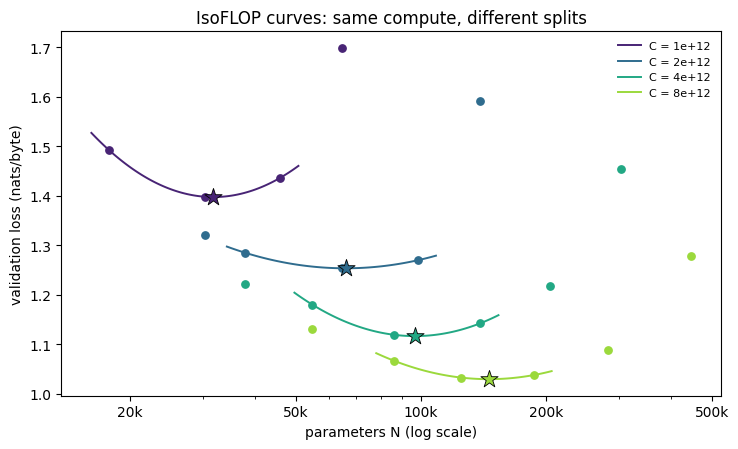
C = 1.0e+12:  N_opt ≈ 32k   D_opt ≈ 5.3M   D/N ≈ 166   L ≈ 1.3975
C = 2.0e+12:  N_opt ≈ 66k   D_opt ≈ 5.1M   D/N ≈ 77   L ≈ 1.2537
C = 4.0e+12:  N_opt ≈ 97k   D_opt ≈ 6.9M   D/N ≈ 71   L ≈ 1.1168
C = 8.0e+12:  N_opt ≈ 146k   D_opt ≈ 9.2M   D/N ≈ 63   L ≈ 1.0298
Each curve is a valley. Left of the bottom, models are too small: they read plenty of data but had no room to use it. Right of the bottom, models are too large for the budget: they had the capacity, but the compute ran out after too few tokens. At this scale, too few tokens means too few optimizer steps. Look at the steps column in the table: the runs on the right wall got little more than a thousand. The star is the balance between the two.
A star only counts if it sits between real runs. A parabola can always be extended past the last point, but its vertex out there is a guess, not a measurement. That is what the bracketing check guards.
Three fits through the stars: best size, best data, and best loss, each against compute.
def power_fit(xs, ys):
    """Fit y = k · x^p in log space. Returns (p, k, r2)."""
    lx, ly = np.log(xs), np.log(ys)
    p, logk = np.polyfit(lx, ly, 1)
    resid = ly - (p * lx + logk)
    r2 = 1 - (resid**2).sum() / ((ly - ly.mean()) ** 2).sum()
    return float(p), float(math.exp(logk)), float(r2)


def loss_fit(cs, ls, floor=None):
    """Fit L(C) = E + A · C^(-alpha). Pass `floor` to fix E instead of fitting it.

    E is found by scanning: for each candidate floor, the rest is a straight line
    in log space, so the scan is exact and needs no optimizer.
    """
    cs, ls = np.asarray(cs), np.asarray(ls)
    floors = np.linspace(0.0, ls.min() * 0.995, 400) if floor is None else np.array([floor])
    best = None
    for e in floors:
        slope, logA = np.polyfit(np.log(cs), np.log(ls - e), 1)
        sse = ((e + np.exp(logA) * cs**slope - ls) ** 2).sum()
        if best is None or sse < best[0]:
            best = (sse, float(e), float(math.exp(logA)), float(-slope))
    return best[1], best[2], best[3]  # E, A, alpha


def frontier_points(optima):
    """The optima a frontier may be fitted to, and whether there are enough."""
    good = [o for o in optima if o["interior"]]
    return (good, True) if len(good) >= 3 else (optima, False)


good, enough_interior = frontier_points(optima)
if not enough_interior:
    # An optimum at the edge of the sampled sizes is a guess, not a measurement.
    # Fall back so the cell still runs, but the fit check will fail.
    print(
        tr(
            "⚠ fewer than three budgets have a bracketed optimum; widen the ratio range",
            "⚠ أقلّ من ثلاث ميزانيات لها حجم أمثل محصور بين تجربتين؛ وسّع مدى النِّسب",
        )
    )
C_fit = np.array([o["C"] for o in good])
L_fit = np.array([o["L_opt"] for o in good])
exponent_a, k_N, frontier_r2 = power_fit(C_fit, [o["N_opt"] for o in good])
exponent_b, k_D, _ = power_fit(C_fit, [o["D_opt"] for o in good])
fitted_E, fit_A, alpha_c = loss_fit(C_fit, L_fit)

a_measured, b_measured, E_frontier = round(exponent_a, 3), round(exponent_b, 3), round(fitted_E, 3)
frontier_r2 = round(frontier_r2, 3) if enough_interior else 0.0
ratio_first = round(good[0]["D_opt"] / good[0]["N_opt"])
ratio_last = round(good[-1]["D_opt"] / good[-1]["N_opt"])
tokens_first_m = round(good[0]["D_opt"] / 1e6, 1)
tokens_last_m = round(good[-1]["D_opt"] / 1e6, 1)

print(
    tr(
        f"N_opt ∝ C^{exponent_a:.3f}   (R² {frontier_r2:.3f})\n"
        f"D_opt ∝ C^{exponent_b:.3f}\n"
        f"L_opt(C) = {fitted_E:.3f} + {fit_A:.3g} · C^-{alpha_c:.3f}\n"
        f"tokens per parameter at the best split: {ratio_first} at the smallest fitted budget, "
        f"{ratio_last} at the largest",
        f"N_opt ∝ C^{exponent_a:.3f}   (R² {frontier_r2:.3f})\n"
        f"D_opt ∝ C^{exponent_b:.3f}\n"
        f"L_opt(C) = {fitted_E:.3f} + {fit_A:.3g} · C^-{alpha_c:.3f}\n"
        f"عدد الرموز لكل معامل عند أفضل تقسيم: {ratio_first} عند أصغر ميزانية، "
        f"و{ratio_last} عند أكبرها",
    )
)
print(
    tr(
        "For comparison: Kaplan et al. reported a ≈ 0.73. Chinchilla reported a ≈ 0.50 "
        "and roughly 20 tokens per parameter.",
        "للمقارنة: نشر Kaplan وزملاؤه a ≈ 0.73. ونشرت ورقة Chinchilla a ≈ 0.50، "
        "ونحو 20 رمزاً لكل معامل.",
    )
)N_opt ∝ C^0.715 (R² 0.974)
D_opt ∝ C^0.285
L_opt(C) = 0.637 + 5.58e+03 · C^-0.322
tokens per parameter at the best split: 166 at the smallest fitted budget, 63 at the largest
For comparison: Kaplan et al. reported a ≈ 0.73. Chinchilla reported a ≈ 0.50 and roughly 20 tokens per parameter.The stars lie close to a straight line in log space: N_opt ∝ C^a, with a = 0.715. Kaplan reported 0.73 and Chinchilla 0.50. Yours sits at the Kaplan end: when the budget doubles, most of the increase goes into parameters.
The second fit shows the other side of the same fact. The best run's token count barely moves: D_opt ∝ C^b, with b = 0.285. It goes from 5.300 million tokens at the smallest budget to 9.200 million at the largest, while the compute doubles several times over. At these budgets a few million tokens is a few thousand optimizer steps. A run seems to need about that many before its size can pay off. Once it has them, extra compute is better spent on parameters.
So tokens per parameter is not a constant here. At the best split it falls from 166 at the smallest budget to 63 at the largest. Chinchilla's 20 was a measurement of their models, their tokenizer and their data, at budgets many orders of magnitude above ours. It does not carry over to this setup, and our numbers would not carry over to theirs. One difference is the unit itself: a byte carries much less information than a tokenizer's token, which usually spans several characters.
The third fit is the loss frontier, L_opt(C) = E + A·C^(−α). It shows : each doubling of compute removes less loss than the one before. It also has a floor, E = 0.637 nats per byte: the level this family of models approaches but would not cross, however large the budget. That floor is the , as these few points see it.
A law that only describes the points it was fitted to is . The reason to fit one is : choosing a model at a budget you have not tried yet. So the next cell commits, in writing, to a model size and a loss for a budget 4× larger than any fitted point. Only then does the following cell train anything at that budget.
Nothing trains here. Note the two predicted numbers before you run the next cell.
# Commit to two numbers BEFORE training: the budget is beyond every fitted point.
C_holdout = budgets[-1] * cfg["holdout_factor"]
N_pred = k_N * C_holdout**exponent_a
L_pred = fitted_E + fit_A * C_holdout ** (-alpha_c)

# The model we would actually build: the family member nearest the predicted size.
holdout_widths = plan_budget(C_holdout)
committed_width = min(
    (w for w in widths if affordable(C_holdout, w)),
    key=lambda w: abs(math.log(sizes[w]["total"] / N_pred)),
)
holdout_widths = sorted({*holdout_widths, committed_width})

predicted_size_k = round(N_pred / 1e3)
predicted_loss = round(L_pred, 4)
committed_params = sizes[committed_width]["total"]
committed_tokens_m = round(C_holdout / (6 * committed_params) / 1e6, 1)

print(
    tr(
        f"held-out budget {C_holdout:.1e} FLOPs ({cfg['holdout_factor']}× the largest fitted budget)\n"
        f"predicted best size  N ≈ {predicted_size_k:,}k → we commit to width {committed_width}: "
        f"{committed_params:,} params on {committed_tokens_m:.1f}M tokens\n"
        f"predicted best loss  {predicted_loss:.4f} nats/byte",
        f"الميزانية المحجوزة {C_holdout:.1e} FLOPs (أي {cfg['holdout_factor']} أضعاف أكبر ميزانية في التوفيق)\n"
        f"أفضل حجم متوقَّع  N ≈ {predicted_size_k:,}k ← نلتزم بالعرض {committed_width}: "
        f"{committed_params:,} معاملاً على {committed_tokens_m:.1f} مليون رمز\n"
        f"أفضل خسارة متوقَّعة  {predicted_loss:.4f} نات لكل بايت",
    )
)held-out budget 3.2e+13 FLOPs (4× the largest fitted budget)
predicted best size N ≈ 418k → we commit to width 124: 420,112 params on 12.7M tokens
predicted best loss 0.8865 nats/byteThe left panel is the new budget's own valley. The two straight blue lines are the numbers you committed to. See how close the valley's bottom comes to each.
# Train the committed model AND its neighbours at the held-out budget, so the
# budget gets a valley of its own. That is what lets us say whether a miss came
# from choosing the wrong size or from the loss curve itself.
t0 = time.time()
holdout_runs = []
for w in holdout_widths:
    loss, tokens = train_run(w, C_holdout / (6 * sizes[w]["total"]))
    holdout_runs.append(run_record(C_holdout, w, loss, tokens))
holdout_minutes = round((time.time() - t0) / 60, 1)
peak_vram_gb = 0.0
if device == "cuda":
    peak_vram_gb = round(torch.cuda.max_memory_allocated() / 1e9, 2)

print_runs(holdout_runs)
held = find_optimum(C_holdout, holdout_runs)
print()
print_optimum(held)

committed_loss = round(next(r["loss"] for r in holdout_runs if r["width"] == committed_width), 4)
best_holdout_loss = round(min(r["loss"] for r in holdout_runs), 4)
measured_size_k = round(held["N_opt"] / 1e3)
holdout_bracketed = held["interior"]
holdout_ratio = round(held["D_opt"] / held["N_opt"])

# Split the miss in two. `size_regret` is what choosing our size cost, compared
# with the best size we tried. `prediction_error_pct` is how far the predicted
# frontier sits from the best loss this budget actually reached.
size_regret = round(committed_loss - best_holdout_loss, 4)
signed_error_pct = round(100 * (L_pred - best_holdout_loss) / best_holdout_loss, 2)
prediction_error_pct = abs(signed_error_pct)
size_ratio = round(N_pred / held["N_opt"], 2)

print(
    tr(
        f"\nsize:  predicted {predicted_size_k:,}k   measured {measured_size_k:,}k   "
        f"(predicted / measured = {size_ratio:.2f})\n"
        f"loss:  predicted {predicted_loss:.4f}   best measured {best_holdout_loss:.4f}   "
        f"(error {signed_error_pct:+.2f}%)\n"
        f"cost of our size choice: {size_regret:.4f} nats/byte   ({holdout_minutes:.1f} min)",
        f"\nالحجم:  المتوقَّع {predicted_size_k:,}k   المقيس {measured_size_k:,}k   "
        f"(المتوقَّع / المقيس = {size_ratio:.2f})\n"
        f"الخسارة:  المتوقَّعة {predicted_loss:.4f}   أفضل خسارة مقيسة {best_holdout_loss:.4f}   "
        f"(الخطأ {signed_error_pct:+.2f}%)\n"
        f"كلفة اختيارنا للحجم: {size_regret:.4f} نات لكل بايت   ({holdout_minutes:.1f} دقيقة)",
    )
)
if device == "cuda":
    print(
        tr(
            f"peak GPU memory {peak_vram_gb:.2f} GB",
            f"ذروة ذاكرة المعالج الرسومي {peak_vram_gb:.2f} غيغابايت",
        )
    )

fig, (ax0, ax1, ax2) = plt.subplots(1, 3, figsize=(13, 4))
cs = np.geomspace(C_fit.min() / 1.5, C_holdout * 1.5, 100)

draw_valley(ax0, held, ORANGE, lab("held-out budget", "الميزانية المحجوزة"))
ax0.axvline(N_pred, color=BLUE, lw=1.2, ls="--", label=lab("predicted size", "الحجم المتوقَّع"))
ax0.axhline(L_pred, color=BLUE, lw=1.2, ls=":", label=lab("predicted loss", "الخسارة المتوقَّعة"))
ax0.set_xscale("log")
log_axis(ax0.xaxis, sizes=True)
ax0.set_xlabel(lab("parameters N", "عدد المعاملات N"))
ax0.set_ylabel(lab("loss (nats/byte)", "الخسارة (نات لكل بايت)"))
ax0.legend(fontsize=8, frameon=False)

ax1.scatter(
    C_fit,
    [o["N_opt"] for o in good],
    color=BLUE,
    zorder=3,
    label=lab("fitted optima", "أفضل الأحجام في التوفيق"),
)
ax1.plot(cs, k_N * cs**exponent_a, color=BLUE, lw=1.2, ls="--", label=f"N ∝ C^{exponent_a:.2f}")
ax1.scatter(
    [C_holdout],
    [held["N_opt"]],
    marker="D",
    color=ORANGE,
    zorder=4,
    label=lab("measured", "المقيس"),
)
ax1.set_xscale("log")
ax1.set_yscale("log")
log_axis(ax1.xaxis)
log_axis(ax1.yaxis, sizes=True)
ax1.set_xlabel(lab("compute C (FLOPs)", "الحوسبة C بوحدات FLOPs"))
ax1.set_ylabel(lab("best size N", "أفضل حجم N"))
ax1.legend(fontsize=8, frameon=False)

ax2.scatter(C_fit, L_fit, color=BLUE, zorder=3, label=lab("fitted optima", "نقاط التوفيق"))
ax2.plot(
    cs,
    fitted_E + fit_A * cs ** (-alpha_c),
    color=BLUE,
    lw=1.2,
    ls="--",
    label=lab("extrapolated frontier", "الحدّ المُستقرَأ"),
)
ax2.scatter(
    [C_holdout],
    [best_holdout_loss],
    marker="D",
    color=ORANGE,
    zorder=4,
    label=lab("measured", "المقيس"),
)
ax2.set_xscale("log")
log_axis(ax2.xaxis)
ax2.set_ylim(bottom=0)
ax2.set_xlabel(lab("compute C (FLOPs)", "الحوسبة C بوحدات FLOPs"))
ax2.set_ylabel(lab("best loss (nats/byte)", "أفضل خسارة (نات لكل بايت)"))
ax2.legend(fontsize=8, frameon=False)
fig.suptitle(
    lab(
        "Fitted on small budgets, tested on a larger one",
        "توفيق على ميزانيات صغيرة، واختبار على ميزانية أكبر",
    )
)
plt.tight_layout()
plt.show() budget C params N tokens D steps D/N loss
3.2e+13 169,936 31.38M 15,324 185 0.9371
3.2e+13 260,736 20.46M 9,988 78 0.9093
3.2e+13 370,736 14.39M 7,024 39 0.9055
3.2e+13 420,112 12.70M 6,199 30 0.9012
3.2e+13 586,672 9.09M 4,439 15 0.9173
3.2e+13 888,352 6.00M 2,931 7 0.9642
3.2e+13 1,296,512 4.11M 2,009 3 1.0303
C = 3.2e+13: N_opt ≈ 434k D_opt ≈ 12.3M D/N ≈ 28 L ≈ 0.9010
size: predicted 418k measured 434k (predicted / measured = 0.96)
loss: predicted 0.8865 best measured 0.9012 (error -1.63%)
cost of our size choice: 0.0000 nats/byte (4.4 min)
peak GPU memory 0.56 GB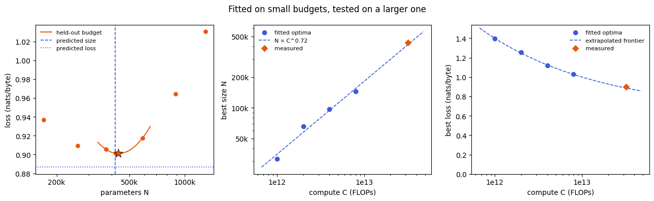
Start with the size. The fit predicted a best size near 418k parameters. The held-out valley's own bottom is near 434k, so the prediction was 0.960 times the measured optimum. The model we committed to scored 0.901, and the best model trained at this budget scored 0.901. The gap between them, 0 nats per byte, is what our choice of size cost.
Look at the left panel to see why that cost stays small. The valley is wide and nearly flat near its bottom, so a size that is somewhat off loses very little. This is also why a rule of thumb for the ratio can be useful even when it is not exact.
Now the loss. The fit predicted 0.886 nats per byte, and the best measured loss is 0.901: an error of -1.630%. A negative sign means the prediction was optimistic.
This is the same reasoning that sized Chinchilla before it was trained, only at a much smaller scale. Train small models, find the bottom of each valley, fit the frontier, extrapolate, and then check the extrapolation against a budget you did not fit.
Chinchilla's Approach 3 uses every run at once instead of only the stars. It fits one surface, L(N, D) = E + A/N^α + B/D^β, and reads the allocation exponent off it as a = β / (α + β). If both methods describe the same reality, they should roughly agree. In the paper they did: 0.49 from the IsoFLOP method and 0.46 from the surface. The surface also makes its own prediction for the held-out budget, so we can score it the same way.
Compare the two exponents, then the two predictions for the held-out budget.
# Chinchilla's third approach: fit one surface L(N, D) = E + A/N^alpha + B/D^beta
# to every fitted run at once, then read the allocation exponent off it.
def fit_surface(rows):
    """Scan the two exponents; solve E, A and B exactly for each pair.

    For fixed alpha and beta the surface is linear in E, A and B, so those three
    come from least squares (on relative error, kept non-negative). Scanning the
    exponents on a grid then finds the best pair with no optimizer to mislead us.
    """
    N = np.array([r["N"] for r in rows], dtype=float)
    D = np.array([r["D"] for r in rows], dtype=float)
    L = np.array([r["loss"] for r in rows])
    ones = np.ones_like(L)
    best = None
    for alpha in np.arange(0.05, 3.0001, 0.025):
        for beta in np.arange(0.05, 3.0001, 0.025):
            X = np.stack([ones, N**-alpha, D**-beta], axis=1) / L[:, None]
            # Drop a term whenever the unconstrained solve would make it negative.
            for cols in ([0, 1, 2], [1, 2], [0, 1], [0, 2]):
                coef = np.linalg.lstsq(X[:, cols], ones, rcond=None)[0]
                if (coef >= 0).all():
                    sse = ((X[:, cols] @ coef - 1) ** 2).sum()
                    if best is None or sse < best[0]:
                        full = np.zeros(3)
                        full[cols] = coef
                        best = (sse, float(alpha), float(beta), full)
                    break
    sse, alpha, beta, (E, A, B) = best
    return {"E": float(E), "A": float(A), "B": float(B), "alpha": alpha, "beta": beta}


def surface_loss(s, N, D):
    return s["E"] + s["A"] / N ** s["alpha"] + s["B"] / D ** s["beta"]


surface = fit_surface(runs)
param_exponent_a = round(surface["beta"] / (surface["alpha"] + surface["beta"]), 3)
param_E = round(surface["E"], 3)

# The surface makes its own prediction for the held-out budget: walk along
# D = C / (6 N) and take the lowest point.
n_grid = np.geomspace(sizes[widths[0]]["total"], sizes[widths[-1]]["total"], 400)
along = surface_loss(surface, n_grid, C_holdout / (6 * n_grid))
surface_size_k = round(float(n_grid[along.argmin()]) / 1e3)
surface_pred = round(float(along.min()), 4)
surface_error_pct = round(100 * (surface_pred - best_holdout_loss) / best_holdout_loss, 2)

print(
    tr(
        f"L(N, D) = {surface['E']:.3f} + {surface['A']:.3g}/N^{surface['alpha']:.3f} "
        f"+ {surface['B']:.3g}/D^{surface['beta']:.3f}\n"
        f"allocation exponent: surface a = β/(α+β) = {param_exponent_a:.3f}"
        f"   ·   IsoFLOP a = {exponent_a:.3f}\n"
        f"irreducible loss E:  surface {param_E:.3f}   ·   frontier {fitted_E:.3f}\n"
        f"held-out budget:     surface predicts N ≈ {surface_size_k:,}k, loss {surface_pred:.4f}"
        f" (error {surface_error_pct:+.2f}%)\n"
        f"                     frontier predicted N ≈ {predicted_size_k:,}k, loss {predicted_loss:.4f}"
        f" (error {signed_error_pct:+.2f}%)\n"
        f"                     measured N ≈ {measured_size_k:,}k, loss {best_holdout_loss:.4f}",
        f"L(N, D) = {surface['E']:.3f} + {surface['A']:.3g}/N^{surface['alpha']:.3f} "
        f"+ {surface['B']:.3g}/D^{surface['beta']:.3f}\n"
        f"أُسّ التوزيع: من السطح a = β/(α+β) = {param_exponent_a:.3f}"
        f"   ·   بطريقة الحوسبة الثابتة a = {exponent_a:.3f}\n"
        f"الخسارة غير القابلة للاختزال E:  من السطح {param_E:.3f}   ·   من الحدّ {fitted_E:.3f}\n"
        f"الميزانية المحجوزة:  يتوقّع السطح N ≈ {surface_size_k:,}k، وخسارة {surface_pred:.4f}"
        f" (الخطأ {surface_error_pct:+.2f}%)\n"
        f"                     وتوقّع الحدّ N ≈ {predicted_size_k:,}k، وخسارة {predicted_loss:.4f}"
        f" (الخطأ {signed_error_pct:+.2f}%)\n"
        f"                     والمقيس N ≈ {measured_size_k:,}k، وخسارة {best_holdout_loss:.4f}",
    )
)L(N, D) = 0.689 + 78.1/N^0.475 + 1.88e+10/D^1.650
allocation exponent: surface a = β/(α+β) = 0.776 · IsoFLOP a = 0.715
irreducible loss E: surface 0.689 · frontier 0.637
held-out budget: surface predicts N ≈ 486k, loss 0.8894 (error -1.31%)
frontier predicted N ≈ 418k, loss 0.8865 (error -1.63%)
measured N ≈ 434k, loss 0.9012The surface gives a = 0.776 and a floor E = 0.689. The IsoFLOP method gave a = 0.715 and E = 0.637. For the held-out budget, the surface predicted a best size of 486k parameters and a loss of 0.889, an error of -1.310%.
The two methods read the same runs, so a gap between them cannot be noise in the training. It comes from what each one assumes. The surface assumes one formula holds for every run, including the runs on the steep right wall of each valley. The IsoFLOP method looks only at the three runs around each bottom, and assumes nothing about the rest.
Here the two agree on the main points. Both give an exponent well above 0.5. Both put the floor at a similar level. And both predict a loss for the held-out budget that is close to the measured one. When two methods with different assumptions reach the same answer, that answer deserves more trust than either fit alone.
Exercise
No model predicts text perfectly, so the real frontier has a floor: the irreducible loss. The fit had to estimate that floor from a handful of points. This cell fixes the floor by hand and refits the rest. It starts at zero, which is a pure power law that keeps falling forever. Before you run it, predict: will it place the held-out loss higher or lower than the fit with a floor did? Then raise E_FLOOR in steps. Watch two numbers: how well the curve still fits the points it was fitted to, and how close it lands at the held-out budget.
# YOUR TURN — the floor you cannot see.
#
# No model predicts text perfectly, so the true loss curve has a floor E > 0.
# The fit above had to guess E from a handful of points. This cell fixes the
# floor by hand and refits the rest. It starts at zero: a pure power law, which
# keeps falling forever. Before you run it, guess: will that place the held-out
# loss higher or lower than the fit with a floor did? Then raise E_FLOOR in
# steps, and watch two numbers: how well the curve still fits the points it was
# fitted to, and how close it lands at the held-out budget.
E_FLOOR = 0.0

_, A_try, alpha_try = loss_fit(C_fit, L_fit, floor=E_FLOOR)
floor_pred = round(E_FLOOR + A_try * C_holdout ** (-alpha_try), 4)
floor_error_pct = round(100 * (floor_pred - best_holdout_loss) / best_holdout_loss, 2)


def worst_fit_error(E, A, alpha):
    """Largest relative error of a frontier curve on the points it was fitted to."""
    return round(100 * float(np.abs((E + A * C_fit ** (-alpha)) / L_fit - 1).max()), 2)


fitted_in_range_pct = worst_fit_error(fitted_E, fit_A, alpha_c)
in_range_error_pct = worst_fit_error(E_FLOOR, A_try, alpha_try)
print(
    tr(
        f"fitted floor E = {fitted_E:.3f}:  on the fitted points, off by at most {fitted_in_range_pct:.2f}%\n"
        f"    held-out prediction {predicted_loss:.4f}  → error {signed_error_pct:+.2f}%\n"
        f"floor fixed at {E_FLOOR}:  on the fitted points, off by at most {in_range_error_pct:.2f}%\n"
        f"    held-out prediction {floor_pred:.4f}  → error {floor_error_pct:+.2f}%",
        f"الأرضية المُوفَّقة E = {fitted_E:.3f}:  أكبر خطأ على نقاط التوفيق {fitted_in_range_pct:.2f}%\n"
        f"    التوقّع للميزانية المحجوزة {predicted_loss:.4f}  ← الخطأ {signed_error_pct:+.2f}%\n"
        f"الأرضية مثبّتة عند {E_FLOOR}:  أكبر خطأ على نقاط التوفيق {in_range_error_pct:.2f}%\n"
        f"    التوقّع للميزانية المحجوزة {floor_pred:.4f}  ← الخطأ {floor_error_pct:+.2f}%",
    )
)A hint is available in the notebook — env.hint(1)
Exercise
This cell refits the frontier using the non-embedding parameter count. Nothing is retrained; only the number written next to each model changes. Before you run it, guess whether the exponent a goes up or down. Then compare it with Kaplan's reported 0.73 and Chinchilla's 0.50.
# YOUR TURN — the bookkeeping.
#
# Kaplan et al. counted parameters WITHOUT the embedding tables; Chinchilla
# counted all of them. This cell refits the frontier with the Kaplan count,
# from the very same training runs. Nothing is retrained. Only the number you
# write next to each model changes. Set COUNT = "total" to get the original back.
COUNT = "non_embedding"

recount, _ = frontier_points(isoflop_optima(runs, count=COUNT))
count_exponent_a, _, count_r2 = power_fit(
    [o["C_count"] for o in recount], [o["N_opt"] for o in recount]
)
count_exponent_a = round(count_exponent_a, 3)
count_ratio_last = round(recount[-1]["D_opt"] / recount[-1]["N_opt"])
print(
    tr(
        f"count={COUNT}:  N_opt ∝ C^{count_exponent_a:.3f}  (R² {count_r2:.3f})   "
        f"tokens/param at the largest budget {count_ratio_last}\n"
        f"count=total:  N_opt ∝ C^{exponent_a:.3f}   tokens/param {ratio_last}",
        f"count={COUNT}:  N_opt ∝ C^{count_exponent_a:.3f}  (R² {count_r2:.3f})   "
        f"رموز لكل معامل عند أكبر ميزانية {count_ratio_last}\n"
        f"count=total:  N_opt ∝ C^{exponent_a:.3f}   رموز لكل معامل {ratio_last}",
    )
)A hint is available in the notebook — env.hint(2)
Both exercises refit the same runs, and both change the answer.
Without a floor, the prediction for the held-out budget is off by -7.860%, against -1.630% with the fitted floor. Yet on the points it was fitted to, the pure power law is never off by more than 1.320%. Inside the fitted range the two curves are hard to tell apart. At a budget 4× further out, they are not. A fit can only be judged by a test outside its range.
Counting parameters like Kaplan moves the exponent from 0.715 to 0.748, with no retraining. The direction makes sense. Embedding tables are a larger share of a small model than of a large one, so removing them shrinks the small models most, and size then appears to grow faster with compute. A later analysis attributes much of the gap between the two papers to this: the earlier law counted non-embedding parameters, at model sizes where embeddings are a large share.
Exercise
PyTorch's default embedding initialisation is much larger than ours. Because the token table is also the output layer, the default starts every run with confident, wrong predictions, and the first steps go to undoing them. This cell re-measures the smallest budget's valley with that default, using the same models and the same seeds. Before you run it, predict which way the best size moves. The cell trains a few more models, so it takes a minute or two.
# YOUR TURN — the handicap.
#
# PyTorch's default embedding init has std 1. Because our token table is also
# the output layer, that starts every run with confident, wrong predictions,
# and the first few hundred steps go to undoing them. A long run can absorb
# that cost; a short run cannot. This cell re-measures the smallest budget's
# valley with INIT_STD = 1.0, using the same sizes and the same seeds as the
# grid. Before you run it, guess which way the best size moves. Set INIT_STD
# back to cfg["init_std"] to recover the grid's own valley.
INIT_STD = 1.0

C_small = budgets[0]
handicap_runs = []
for w in plan_budget(C_small):
    loss, tokens = train_run(w, C_small / (6 * sizes[w]["total"]), init_std=INIT_STD)
    handicap_runs.append(run_record(C_small, w, loss, tokens))
handicapped = find_optimum(C_small, handicap_runs)
fair = optima[0]

print_runs(handicap_runs)
fair_size_k, handicap_size_k = round(fair["N_opt"] / 1e3), round(handicapped["N_opt"] / 1e3)
fair_ratio, handicap_ratio = (
    round(fair["D_opt"] / fair["N_opt"]),
    round(handicapped["D_opt"] / handicapped["N_opt"]),
)
handicap_cost = round(handicapped["L_opt"] - fair["L_opt"], 4)
print(
    tr(
        f"\nbudget {C_small:.1e}, init std {cfg['init_std']}:  best size {fair_size_k}k   "
        f"tokens/param {fair_ratio}   loss {fair['L_opt']:.4f}\n"
        f"budget {C_small:.1e}, init std {INIT_STD}:  best size {handicap_size_k}k   "
        f"tokens/param {handicap_ratio}   loss {handicapped['L_opt']:.4f}",
        f"\nالميزانية {C_small:.1e}، انحراف التهيئة {cfg['init_std']}:  أفضل حجم {fair_size_k}k   "
        f"رموز لكل معامل {fair_ratio}   الخسارة {fair['L_opt']:.4f}\n"
        f"الميزانية {C_small:.1e}، انحراف التهيئة {INIT_STD}:  أفضل حجم {handicap_size_k}k   "
        f"رموز لكل معامل {handicap_ratio}   الخسارة {handicapped['L_opt']:.4f}",
    )
)

fig, ax = plt.subplots(figsize=(7.5, 4.2))
draw_valley(ax, fair, BLUE, lab(f"init std {cfg['init_std']}", f"انحراف التهيئة {cfg['init_std']}"))
draw_valley(ax, handicapped, ORANGE, lab(f"init std {INIT_STD}", f"انحراف التهيئة {INIT_STD}"))
ax.set_xscale("log")
log_axis(ax.xaxis, sizes=True)
ax.set_xlabel(lab("parameters N (log scale)", "عدد المعاملات N (مقياس لوغاريتمي)"))
ax.set_ylabel(lab("validation loss (nats/byte)", "خسارة التحقق (نات لكل بايت)"))
ax.set_title(
    lab(
        "Same budget, same sizes, different starting point",
        "الميزانية نفسها والأحجام نفسها، ونقطة بداية مختلفة",
    )
)
ax.legend(fontsize=8, frameon=False)
plt.tight_layout()
plt.show()A hint is available in the notebook — env.hint(3)
With the default initialisation, the best size at the smallest budget moved from 32k to 25k parameters, and the best loss rose by 0.114 nats per byte. Nothing about the models or the data changed.
The handicap is the same for every run: some steps wasted at the start. But a short run loses a larger share of its training to it than a long one does. At a fixed budget, the short runs are the large models. So the large models suffer most, and the bottom of the valley slides toward smaller ones.
This is the kind of detail that separates the two papers. The Chinchilla authors argue that the earlier setup made training on fewer tokens look worse than it was, and that this bias shaped the earlier law. A scaling law is a property of a whole measurement setup: the models, the data, the tokenizer, the optimizer, the initialisation and the bookkeeping. Change one of them and you should measure again.
The first two checks make sure the grid measured something. The last two check what you did with it.
learned_ok = env.check("runs-learned", worst_margin)
bracketed_ok = env.check("optima-bracketed", bracketed_share)
frontier_ok = env.check("frontier-fit", frontier_r2)
prediction_ok = env.check("prediction-error", prediction_error_pct)✓ Smallest gain over the unigram baseline across all grid runs, in nats per byte: 1.387 (needs ≥ 0.8)
✓ Share of fitted budgets whose best model size has a smaller and a larger run on either side: 1 (needs ≥ 0.75)
✓ How well a power law describes best size against compute (coefficient of determination, in log space): 0.974 (needs ≥ 0.9)
✓ Gap between the predicted loss and the best loss measured at the held-out budget, as a percentage: 1.63 (needs ≤ 10)receipt = env.receipt()Workshop complete.
Completion code: AZ-██████████
Paste it on the workshop's page on Azimuth to record it.What should stay with you is the procedure rather than any one exponent. Fix the compute, vary the split, find the bottom of each valley, fit a line through the bottoms, and test the line on a budget you did not fit. The same procedure was used to plan models with billions of parameters.
On this setup it gave N ∝ C^0.715, and 28 bytes per parameter at the held-out budget. Chinchilla found 0.50, and 20 tokens per parameter. Neither pair of numbers is wrong. Each is what a measured law looks like for one setup, and the measurement is something you can now repeat yourself.
Terms in this workshop
- Scaling Lawقانون التحجيم
- Compute-Optimalالأمثل حوسبياً
- Chinchilla Scalingمعايير تشينشيلا للتوسع
- Model Scaleحجم النموذج
- Compute Budgetالميزانية الحوسبية
- Lossالفقد
- Loss functionدالة الخسارة
- Cross-Entropy Lossفقد الإنتروبيا التقاطعية
- Datasetمجموعة البيانات
- Data Efficiencyكفاءة البيانات
- Generalizationالتعميم
- Extrapolation (Statistical)الاستقراء الإحصائي
- Interpolation (Statistical)الاستيفاء الإحصائي
- Power Lawقانون القدرة
- Model Efficiency & Scalingكفاءة النماذج وتوسيع النطاق