Minds & LifeintermediateGPU~55 minColab
Grid Cells From a Network That Was Never Asked
خلايا الشبكة: نمطٌ سداسي لم يطلبه أحد
A representation nobody asked for is still an answer to a question somebody asked
A rat in the dark still knows where it is. It feels its own speed and turning and keeps a running sum: . In 2005, recordings from the rat's entorhinal cortex found neurons that fire at the corners of a triangular lattice laid across the whole room. They were named grid cells, and nothing in the rat's world is hexagonal. Here you hand a small recurrent network the same problem: velocity in, "where am I?" out. Hexagons are never mentioned. Then you open the network and draw where each hidden unit fires. You also train a twin that differs in one detail only, to find out what the hexagons were really a response to.
The goal
Both networks learn to track their own position from velocity alone, and the centre-surround network does it less precisely. Its grid scores still sit above its Gaussian twin's as a whole, and in this seed a clear share of its units become stable hexagonal maps. Across seven seeds that share ranged from 1% to 22%: the lean toward a lattice held, and the lattice itself did not.
Colab opens a read-only copy. Save a copy to Drive to keep your edits.
The notebook needs a keyboard — best opened on a desktop.
The papers behind this
Close your eyes and walk three steps forward, turn left, walk two more. You still have a fair idea where the door is. Nothing told you; you integrated your own motion. Animals do this constantly, and in the entorhinal cortex of the rat some of the neurons involved have a startling signature: plotted against position, each one fires at the vertices of a triangular lattice that tiles the entire floor.
This workshop asks whether an artificial network, given only the same problem, arrives at the same answer — and then asks the harder question of what exactly made it do so.
Confirm the profile and the code hash; everything below is sized from that profile.
import azimuth_nb as azimuth

env = azimuth.setup(SLUG, lang=LANG, profile=PROFILE)Grid Cells From a Network That Was Never Asked
Tesla T4 · 14.6 GB · 12.7 GB RAM · PyTorch 2.11.0+cu128
profile: free
ready · seed=17, box_m=2.2, place_cells=512, place_sigma_m=0.12, surround_scale=2, hidden_units=4096, seq_len=20, batch=200, train_steps=30000, learning_rate=0.0001, weight_decay=0.0001, log_every=2000, map_res=20, eval_batches=25, grid_score_cut=0.3, stability_min=0.5, ring_max=0.7, units_shown=25
code · e249e89f5ca00d87The network's output is not a pair of coordinates. It predicts the activity of 512 simulated place cells scattered over a 2.2-metre box, each most active near its own centre. The workshop trains two versions that differ in the shape of that tuning. In one, each is a plain Gaussian bump. In the other, the bump is ringed by a shallow zone of suppression — a centre-surround profile. Walks, starting weights, network and training schedule are identical. Hold on to that single difference; the rest of the workshop turns on it.
Left: six simulated walks over grey place-cell centres; when a walk reaches a wall it slows and slides along it. Right: one place cell's activity along a line through its centre, orange for centre-surround and blue for Gaussian. The orange curve never goes negative. It sits on a raised floor and is notched down to zero in a ring around the peak, and that ring is the surround. Because the code must stay non-negative and sum to one, about three quarters of the centre-surround code is that nearly flat floor, which is why this network's loss will barely move.
import math

import matplotlib.pyplot as plt
import numpy as np
import torch

assert torch.__version__, "torch comes with the runtime; it is never installed here"
device = torch.device("cuda" if torch.cuda.is_available() else "cpu")
cfg = env.cfg
BOX = cfg["box_m"]
DT = 0.02  # seconds per step
torch.manual_seed(cfg["seed"])

# One fixed set of place-cell centres, shared by both networks.
centers = (
    torch.rand(cfg["place_cells"], 2, generator=torch.Generator().manual_seed(cfg["seed"])) - 0.5
) * BOX
centers = centers.to(device)


def make_trajectories(rng, batch, steps, box=BOX):
    """Smooth random walks that turn away from walls. Returns positions (batch, steps+1, 2)."""
    sigma_turn = 11.52  # rad/s, rotational velocity spread
    speed_scale = 0.13 * 2 * math.pi  # m/s, Rayleigh scale of forward speed
    border = 0.03
    pos = np.zeros((batch, steps + 1, 2))
    pos[:, 0] = rng.uniform(-box / 2, box / 2, (batch, 2))
    heading = rng.uniform(0, 2 * math.pi, batch)
    turns = rng.normal(0, sigma_turn, (batch, steps))
    speeds = rng.rayleigh(speed_scale, (batch, steps))
    for t in range(steps):
        x, y = pos[:, t, 0], pos[:, t, 1]
        dists = np.stack([box / 2 - x, box / 2 - y, box / 2 + x, box / 2 + y])
        wall_angle = dists.argmin(0) * math.pi / 2
        toward = np.mod(heading - wall_angle + math.pi, 2 * math.pi) - math.pi
        near = (dists.min(0) < border) & (np.abs(toward) < math.pi / 2)
        v = np.where(near, 0.25, 1.0) * speeds[:, t]
        heading = (
            heading
            + np.where(near, np.sign(toward) * (math.pi / 2 - np.abs(toward)), 0.0)
            + DT * turns[:, t]
        )
        pos[:, t + 1] = pos[:, t] + (v * DT)[:, None] * np.stack(
            [np.cos(heading), np.sin(heading)], -1
        )
    return pos


def place_code(pos, surround):
    """Population activity of the place cells at positions (..., 2). Sums to 1 over cells.

    surround=None gives plain Gaussian bumps. surround=s subtracts a wider bump
    (variance scaled by s): a centre that excites, ringed by a zone that inhibits.
    """
    d2 = ((pos[..., None, :] - centers) ** 2).sum(-1)
    width2 = cfg["place_sigma_m"] ** 2
    out = torch.softmax(-d2 / (2 * width2), -1)
    if surround is not None:
        out = out - torch.softmax(-d2 / (2 * surround * width2), -1)
        out = out - out.min(-1, keepdim=True).values
        out = out / out.sum(-1, keepdim=True)
    return out


# Picture the task: a few walks, and one place cell's tuning under each target.
rng = np.random.default_rng(cfg["seed"])
walks = make_trajectories(rng, 6, 200)
fig, (ax_walk, ax_tune) = plt.subplots(1, 2, figsize=(9, 4))
c = centers.cpu().numpy()
ax_walk.scatter(c[:, 0], c[:, 1], s=4, color="0.8")
for w in walks:
    ax_walk.plot(w[:, 0], w[:, 1], lw=1)
ax_walk.set_xlim(-BOX / 2, BOX / 2)
ax_walk.set_ylim(-BOX / 2, BOX / 2)
ax_walk.set_aspect("equal")

nearest = int((centers**2).sum(-1).argmin())  # the place cell closest to the middle
xs = torch.linspace(-BOX / 2, BOX / 2, 400, device=device)
line = torch.stack([xs, torch.full_like(xs, centers[nearest, 1].item())], -1)
for surround, colour in [(cfg["surround_scale"], "tab:orange"), (None, "tab:blue")]:
    tuning = place_code(line, surround)[:, nearest].cpu().numpy()
    ax_tune.plot(xs.cpu().numpy(), tuning / tuning.max(), color=colour, lw=2)
ax_tune.axhline(0, color="0.6", lw=0.8)
ax_tune.set_ylim(-0.3, 1.1)
plt.tight_layout()
plt.show()

if env.lang == "ar":
    hardware = "بطاقة رسوميات" if device.type == "cuda" else "المعالج المركزي"
    print(f"الساحة {BOX} م × {BOX} م · {cfg['place_cells']} خلية مكان · التشغيل على {hardware}")
else:
    print(f"arena {BOX} m × {BOX} m · {cfg['place_cells']} place cells · device: {device}")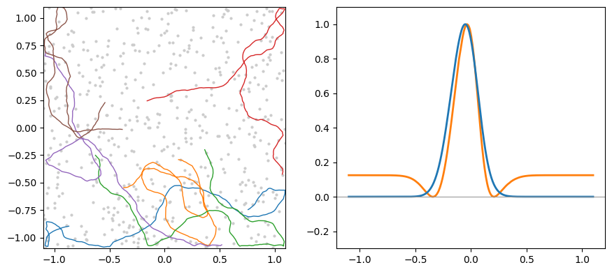
arena 2.2 m × 2.2 m · 512 place cells · device: cudaThe starts from the place-cell code of the starting point. From then on the network receives one thing per step: how far it moved in x and y. To predict the place code 20 steps on, it must accumulate those movements inside its hidden state. The loss compares predicted and true place-cell activity. It contains no term about spatial structure, periodicity, or angles.
An encoder for the starting place, a ReLU recurrent layer, and a linear readout — nothing more.
from torch import nn


class PathIntegrator(nn.Module):
    """Velocity in, place-cell prediction out. The hidden layer is never told what to be."""

    def __init__(self, n_place, n_hidden):
        super().__init__()
        self.encoder = nn.Linear(
            n_place, n_hidden, bias=False
        )  # starting place -> first hidden state
        self.rnn = nn.RNN(2, n_hidden, nonlinearity="relu", bias=False, batch_first=True)
        self.decoder = nn.Linear(n_hidden, n_place, bias=False)

    def hidden(self, velocity, start_code):
        states, _ = self.rnn(velocity, self.encoder(start_code)[None])
        return states

    def forward(self, velocity, start_code):
        return self.decoder(self.hidden(velocity, start_code))


def decode(logits):
    """Position estimate: the mean centre of the three most active predicted place cells."""
    return centers[logits.topk(3, dim=-1).indices].mean(-2)


def batch_tensors(pos, surround):
    pos = torch.as_tensor(pos, dtype=torch.float32, device=device)
    velocity = pos[:, 1:] - pos[:, :-1]
    return pos, velocity, place_code(pos[:, 0], surround), place_code(pos[:, 1:], surround)


params = sum(
    p.numel() for p in PathIntegrator(cfg["place_cells"], cfg["hidden_units"]).parameters()
)
if env.lang == "ar":
    print(f"{cfg['hidden_units']} وحدة مخفية · {params / 1e6:.1f} مليون معامل")
else:
print(f"{cfg['hidden_units']} hidden units · {params / 1e6:.1f}M parameters")4096 hidden units · 21.0M parametersWatch the position error decoded from the predicted place cells, not the loss, which barely moves. Expect a long plateau near a metre. In the reference run the error first fell below half a metre at step 18,000 and ended at 9.400 cm. Every one of seven seeds tested broke through, the measured ones between fourteen and twenty thousand steps. Do not stop the cell while the error is flat: position error is the whole of what the network is rewarded for, and the break comes late.
import time


def train(surround):
    torch.manual_seed(cfg["seed"])  # identical initial weights for both networks
    rng = np.random.default_rng(cfg["seed"])  # identical trajectories for both networks
    model = PathIntegrator(cfg["place_cells"], cfg["hidden_units"]).to(device)
    opt = torch.optim.Adam(model.parameters(), lr=cfg["learning_rate"])
    # Half precision for the recurrent arithmetic on a GPU. A T4 in full precision
    # ran 6.4 steps/s here, almost all of it matrix multiplication. The loss stays
    # in full precision, and the scaler keeps its very small gradients from
    # rounding to zero.
    amp = device.type == "cuda"
    scaler = torch.amp.GradScaler("cuda", enabled=amp)
    if device.type == "cuda":
        torch.cuda.reset_peak_memory_stats()
    history, started = [], time.time()
    for step in range(1, cfg["train_steps"] + 1):
        pos, velocity, start, target = batch_tensors(
            make_trajectories(rng, cfg["batch"], cfg["seq_len"]), surround
        )
        with torch.autocast(device_type=device.type, dtype=torch.float16, enabled=amp):
            logits = model(velocity, start)
        logits = logits.float()
        loss = -(target * torch.log_softmax(logits, -1)).sum(-1).mean()
        loss = loss + cfg["weight_decay"] * (model.rnn.weight_hh_l0**2).sum()
        opt.zero_grad(set_to_none=True)
        scaler.scale(loss).backward()
        scaler.step(opt)
        scaler.update()
        if step % cfg["log_every"] == 0 or step == cfg["train_steps"]:
            with torch.no_grad():
                err_cm = 100 * (decode(logits) - pos[:, 1:]).norm(dim=-1).mean().item()
            history.append((step, loss.item(), err_cm))
            rate = step / (time.time() - started)
            if env.lang == "ar":
                print(
                    f"خطوة {step:>6} · الخسارة {loss.item():.3f} · خطأ الموضع {err_cm:.1f} سم · {rate:.1f} خطوة/ث"
                )
            else:
                print(
                    f"step {step:>6} · loss {loss.item():.3f} · position error {err_cm:.1f} cm · {rate:.1f} steps/s"
                )
    peak = torch.cuda.max_memory_allocated() / 2**30 if device.type == "cuda" else 0.0
    return model.eval(), np.array(history), time.time() - started, peak


dog_model, dog_history, dog_seconds, dog_peak_gb = train(cfg["surround_scale"])
train_minutes_dog = round(dog_seconds / 60, 1)
peak_vram_gb = round(dog_peak_gb, 2)
dog_final_error_cm = round(float(dog_history[-1, 2]), 1)
# The first logged step below half a metre: where the plateau broke, if it did.
broke = dog_history[dog_history[:, 2] < 50, 0]
plateau_break_step = int(broke[0]) if len(broke) else Nonestep 2000 · loss 6.238 · position error 108.9 cm · 24.1 steps/s
step 4000 · loss 6.238 · position error 112.1 cm · 23.7 steps/s
step 6000 · loss 6.238 · position error 111.7 cm · 23.5 steps/s
step 8000 · loss 6.238 · position error 105.0 cm · 23.5 steps/s
step 10000 · loss 6.238 · position error 104.1 cm · 23.5 steps/s
step 12000 · loss 6.235 · position error 94.0 cm · 23.5 steps/s
step 14000 · loss 6.232 · position error 89.6 cm · 23.6 steps/s
step 16000 · loss 6.222 · position error 69.5 cm · 23.7 steps/s
step 18000 · loss 6.210 · position error 39.4 cm · 23.8 steps/s
step 20000 · loss 6.197 · position error 19.2 cm · 23.8 steps/s
step 22000 · loss 6.190 · position error 15.6 cm · 23.8 steps/s
step 24000 · loss 6.186 · position error 13.2 cm · 23.9 steps/s
step 26000 · loss 6.182 · position error 11.3 cm · 23.9 steps/s
step 28000 · loss 6.182 · position error 11.2 cm · 23.9 steps/s
step 30000 · loss 6.181 · position error 9.4 cm · 23.9 steps/sThe same walks in the same order, from the same starting weights. In the plot, the horizontal axis is training steps and the vertical one is position error in centimetres. The blue curve drops within a few thousand steps; the orange one gets there much later and settles higher. If the blue one never comes down, the twin did not learn the task and nothing later about it means anything.
control_model, control_history, control_seconds, _ = train(None)
train_minutes_control = round(control_seconds / 60, 1)

fig, ax = plt.subplots(figsize=(6, 3.5))
ax.plot(dog_history[:, 0], dog_history[:, 2], color="tab:orange", lw=2)
ax.plot(control_history[:, 0], control_history[:, 2], color="tab:blue", lw=2)
ax.set_ylim(bottom=0)  # zero-based: both curves must visibly reach the floor
plt.tight_layout()
plt.show()step 2000 · loss 3.572 · position error 12.2 cm · 24.6 steps/s
step 4000 · loss 3.451 · position error 10.0 cm · 24.7 steps/s
step 6000 · loss 3.200 · position error 5.2 cm · 24.7 steps/s
step 8000 · loss 3.134 · position error 5.1 cm · 24.7 steps/s
step 10000 · loss 3.092 · position error 4.4 cm · 24.7 steps/s
step 12000 · loss 3.106 · position error 4.4 cm · 24.7 steps/s
step 14000 · loss 3.100 · position error 4.4 cm · 24.7 steps/s
step 16000 · loss 3.119 · position error 4.4 cm · 24.7 steps/s
step 18000 · loss 3.071 · position error 4.6 cm · 24.7 steps/s
step 20000 · loss 3.105 · position error 4.3 cm · 24.7 steps/s
step 22000 · loss 3.082 · position error 4.2 cm · 24.7 steps/s
step 24000 · loss 3.084 · position error 4.2 cm · 24.7 steps/s
step 26000 · loss 3.113 · position error 4.4 cm · 24.7 steps/s
step 28000 · loss 3.070 · position error 4.3 cm · 24.7 steps/s
step 30000 · loss 3.097 · position error 4.5 cm · 24.7 steps/s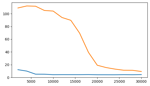
To see what a hidden unit represents, walk the trained network through thousands of fresh trajectories and average that unit's activity in each square of a 20×20 floor grid. The result is its firing map. To score it, correlate the map with shifted copies of itself, which turns any repeating pattern into a ring of peaks around the centre. Rotate that picture. A hexagonal lattice matches itself at 60° and 120° and clashes at 30°, 90° and 150°; the grid score is the gap between the two. Squares and stripes score near or below zero.
Skill compares each network with a guess that never leaves the starting point: 1 is perfect, 0 learned nothing. Both must be well above zero before any map below is worth reading. They will not be equal. The Gaussian twin navigates more precisely, 0.771 against 0.484 in the reference run, and that gap matters for everything that follows.
@torch.no_grad()
def survey(model, surround, seq_len, skip=0):
    """Walk the trained network through fresh trajectories.

    Returns (rate maps [units, res, res], stability [units], decoding skill,
    error in cm, error in cm of always guessing the box centre).
    Only steps at index >= skip are binned and scored. Skill = 1 - model error /
    error of a guess that never moves from the starting point, so 0 means "did
    not integrate". That guess gets worse as walks get longer, so skill is only
    comparable between walks of the same length; the centimetre errors are not.
    Stability correlates the maps built from two halves of the walks: a real map
    agrees with itself, noise does not.
    """
    res = cfg["map_res"]
    rng = np.random.default_rng(cfg["seed"] + 1)  # unseen trajectories, same for both networks
    sums = torch.zeros(2, res * res, cfg["hidden_units"], device=device)
    counts = torch.zeros(2, res * res, device=device)
    model_err, still_err, centre_err = 0.0, 0.0, 0.0
    for batch in range(cfg["eval_batches"]):
        pos, velocity, start, _ = batch_tensors(
            make_trajectories(rng, cfg["batch"], seq_len), surround
        )
        states = model.hidden(velocity, start)[:, skip:]
        where = pos[:, 1 + skip :]
        model_err += (decode(model.decoder(states)) - where).norm(dim=-1).mean().item()
        still_err += (pos[:, :1] - where).norm(dim=-1).mean().item()
        centre_err += where.norm(dim=-1).mean().item()
        cell = ((where + BOX / 2) / BOX * res).long().clamp(0, res - 1)
        index = (cell[..., 0] * res + cell[..., 1]).reshape(-1)
        half = batch % 2
        sums[half].index_add_(0, index, states.reshape(-1, states.shape[-1]))
        counts[half].index_add_(0, index, torch.ones_like(index, dtype=torch.float32))
    maps = (sums.sum(0) / counts.sum(0).clamp(min=1)[:, None]).T.reshape(-1, res, res).cpu().numpy()
    halves = sums / counts.clamp(min=1)[..., None]  # (2, bins, units)
    seen = (counts > 0).all(0)
    a, b = halves[0][seen], halves[1][seen]
    a, b = a - a.mean(0), b - b.mean(0)
    stability = (
        ((a * b).sum(0) / ((a * a).sum(0) * (b * b).sum(0)).sqrt().clamp(min=1e-12)).cpu().numpy()
    )
    per_batch_cm = 100 / cfg["eval_batches"]
    return (
        maps,
        stability,
        1 - model_err / still_err,
        model_err * per_batch_cm,
        centre_err * per_batch_cm,
    )


dog_maps, dog_stability, dog_skill, dog_err_cm, _ = survey(
    dog_model, cfg["surround_scale"], cfg["seq_len"]
)
control_maps, control_stability, control_skill, control_err_cm, _ = survey(
    control_model, None, cfg["seq_len"]
)
dog_skill, control_skill = round(dog_skill, 3), round(control_skill, 3)

if env.lang == "ar":
    print(
        f"مهارة تكامل المسار · هدف المركز والمحيط {dog_skill:.3f} · الهدف الغاوسي {control_skill:.3f}"
    )
    print(
        f"خطأ الموضع · هدف المركز والمحيط {dog_err_cm:.1f} سم · الهدف الغاوسي {control_err_cm:.1f} سم"
    )
else:
    print(
        f"path-integration skill · centre-surround {dog_skill:.3f} · Gaussian {control_skill:.3f}"
    )
    print(
        f"position error · centre-surround {dog_err_cm:.1f} cm · Gaussian {control_err_cm:.1f} cm"
)path-integration skill · centre-surround 0.484 · Gaussian 0.771
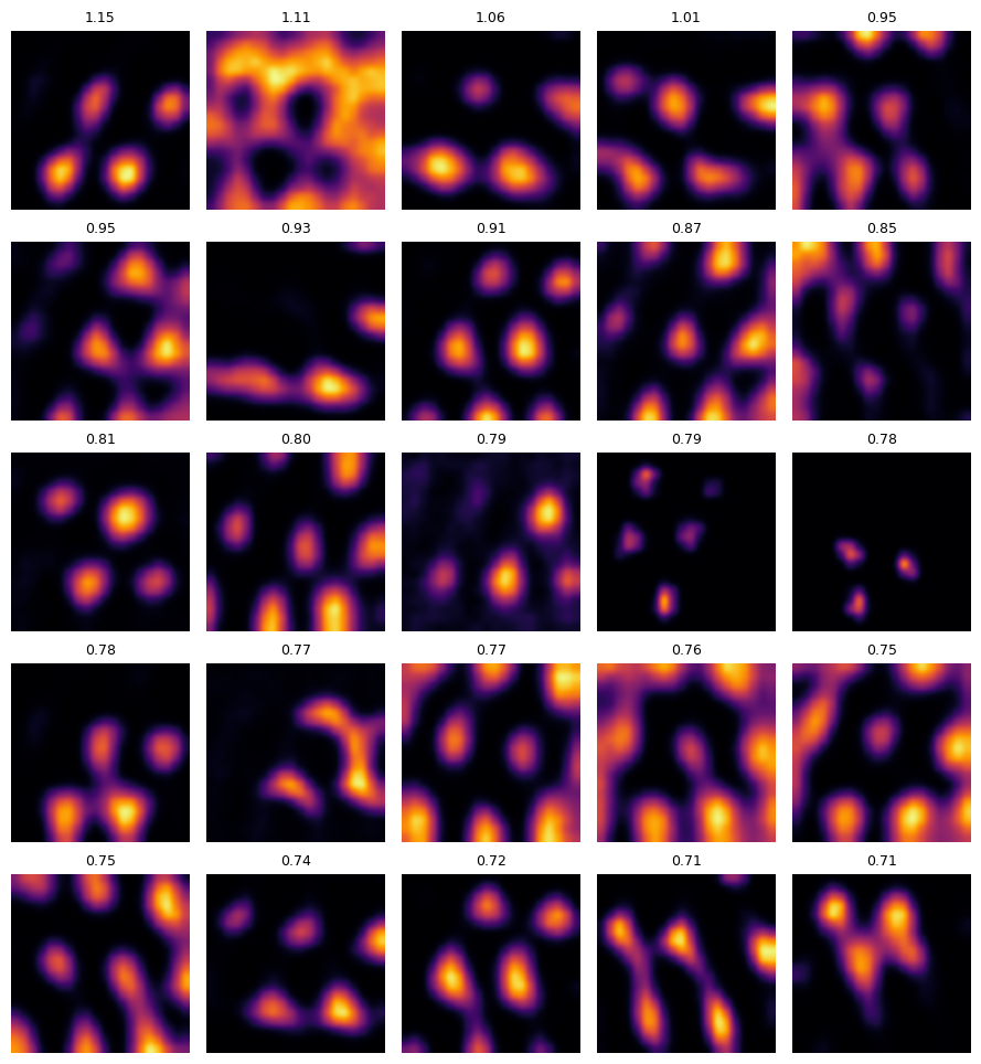
position error · centre-surround 10.0 cm · Gaussian 4.4 cmThe 25 highest-scoring hidden units of the centre-surround network, each drawn over the floor of the box, with its grid score above. Look for bumps arranged in triangles — every unit with its own spacing, orientation and offset. At 20×20 bins the maps are coarse, and a lattice this wide fits only a few periods in the box, so some units show just three or four bumps. The printed line underneath matters as much as the picture. Before training, the same network draws speckled maps, and speckle can score above 1 by pure chance. So a grid unit must also draw the same map from two separate halves of the walks, which a lattice does and speckle never does. This seed is one of the stronger ones; the closing section says how the other seeds went.
def autocorrelogram(maps):
    """Normalised spatial autocorrelation of each map, shape (units, 2*res-1, 2*res-1)."""
    n, res, _ = maps.shape
    size = 2 * res - 1
    x = np.zeros((n, size, size))
    x[:, :res, :res] = maps - maps.mean(axis=(1, 2), keepdims=True)
    ones = np.zeros((1, size, size))
    ones[:, :res, :res] = 1.0

    def xcorr(a, b):
        return np.fft.fftshift(
            np.real(np.fft.ifft2(np.fft.fft2(a) * np.conj(np.fft.fft2(b)))), axes=(1, 2)
        )

    overlap = np.round(xcorr(ones, ones))
    s_a, s_b = xcorr(x, ones), xcorr(ones, x)
    s_ab, s_aa, s_bb = xcorr(x, x), xcorr(x**2, ones), xcorr(ones, x**2)
    num = overlap * s_ab - s_a * s_b
    den = np.sqrt(
        np.clip(overlap * s_aa - s_a**2, 0, None) * np.clip(overlap * s_bb - s_b**2, 0, None)
    )
    sac = np.where((den > 1e-12) & (overlap >= 20), num / np.maximum(den, 1e-12), 0.0)
    return sac  # zero lag sits at index res-1 on both axes


def rotate(images, degrees):
    """Bilinear rotation about the centre, keeping the frame."""
    _, h, w = images.shape
    theta = math.radians(degrees)
    yy, xx = np.mgrid[0:h, 0:w].astype(float)
    cy, cx = (h - 1) / 2, (w - 1) / 2
    src_x = math.cos(theta) * (xx - cx) + math.sin(theta) * (yy - cy) + cx
    src_y = -math.sin(theta) * (xx - cx) + math.cos(theta) * (yy - cy) + cy
    x0, y0 = np.floor(src_x).astype(int), np.floor(src_y).astype(int)
    fx, fy = src_x - x0, src_y - y0
    out = np.zeros_like(images)
    for dy, dx, weight in [
        (0, 0, (1 - fx) * (1 - fy)),
        (0, 1, fx * (1 - fy)),
        (1, 0, (1 - fx) * fy),
        (1, 1, fx * fy),
    ]:
        yi, xi = y0 + dy, x0 + dx
        inside = (yi >= 0) & (yi < h) & (xi >= 0) & (xi < w)
        out += images[:, yi.clip(0, h - 1), xi.clip(0, w - 1)] * (weight * inside)
    return out


def grid_scores(maps):
    """Sixfold symmetry of each map: min(r60, r120) - max(r30, r90, r150), best over ring sizes."""
    sac = autocorrelogram(maps)
    n, size, _ = sac.shape
    res = maps.shape[1]
    r = np.hypot(*(np.mgrid[0:size, 0:size] - (size - 1) / 2))
    rotated = {a: rotate(sac, a).reshape(n, -1) for a in (30, 60, 90, 120, 150)}
    flat = sac.reshape(n, -1)
    best = np.full(n, -np.inf)
    # Rings stop at ring_max of the map width. Beyond it two copies of the map
    # barely overlap, the autocorrelogram is noise, and in the first T4 run that
    # noise gave single blobs scores above 1.1. The cap keeps full sensitivity to
    # lattices up to 0.7 of the box apart.
    for outer in np.linspace(0.4, cfg["ring_max"], 10):
        ring = ((r >= 0.2 * res) & (r <= outer * res)).reshape(-1)
        a = flat[:, ring] - flat[:, ring].mean(1, keepdims=True)
        corr = {}
        for angle, rot in rotated.items():
            b = rot[:, ring] - rot[:, ring].mean(1, keepdims=True)
            corr[angle] = (a * b).sum(1) / np.sqrt((a**2).sum(1) * (b**2).sum(1) + 1e-12)
        score = np.minimum(corr[60], corr[120]) - np.maximum(
            np.maximum(corr[30], corr[90]), corr[150]
        )
        best = np.maximum(best, score)
    return best, sac


def show_maps(maps, scores, count, cmap):
    order = np.argsort(-scores)[:count]  # callers pass unstable units as -inf
    cols = math.ceil(math.sqrt(count))
    rows = math.ceil(count / cols)
    _, axes = plt.subplots(rows, cols, figsize=(1.8 * cols, 1.95 * rows))
    for ax, unit in zip(axes.ravel()[: len(order)], order, strict=True):
        ax.imshow(maps[unit].T, origin="lower", cmap=cmap, interpolation="gaussian")
        ax.set_title(f"{scores[unit]:.2f}", fontsize=9)
    for ax in axes.ravel():
        ax.axis("off")
    plt.tight_layout()
    plt.show()
    return order


def grid_units(maps, scores, stability):
    """A grid unit scores above the cut AND draws the same map from both halves of the walks.

    Returns (mask over units, percent of active units)."""
    active = maps.std(axis=(1, 2)) > 1e-6  # silent units have no map to score
    mask = active & (scores > cfg["grid_score_cut"]) & (stability > cfg["stability_min"])
    return mask, round(100 * float(mask[active].mean()), 1)


# The null. In the same network before training, maps are speckle, and speckle
# can score above 1 by pure chance: on T4 runs about 15% of untrained units
# cleared a score of 0.3, as many as in the trained network. Speckle cannot
# repeat itself across two halves of the data, so the stability test removes it.
torch.manual_seed(cfg["seed"])
untrained = PathIntegrator(cfg["place_cells"], cfg["hidden_units"]).to(device).eval()
untrained_maps, untrained_stability, *_ = survey(untrained, cfg["surround_scale"], cfg["seq_len"])
_, grid_percent_untrained = grid_units(
    untrained_maps, grid_scores(untrained_maps)[0], untrained_stability
)

dog_scores, dog_sac = grid_scores(dog_maps)
control_scores, _ = grid_scores(control_maps)
dog_grid, grid_percent_dog = grid_units(dog_maps, dog_scores, dog_stability)
control_grid, grid_percent_control = grid_units(control_maps, control_scores, control_stability)
active_dog = dog_maps.std(axis=(1, 2)) > 1e-6
active_control = control_maps.std(axis=(1, 2)) > 1e-6
grid_advantage_points = round(grid_percent_dog - grid_percent_control, 1)


# The whole distributions, not just their tails. Across seeds the share of grid
# units varied twentyfold, but the centre-surround median sat above the Gaussian
# twin's in every seed where both were measured, including the weakest.
# Medians are over STABLE units. Over all active units, untrained weights alone
# give a gap of about 0.14, because the start code shifts the speckle's scores;
# speckle is never stable, so an untrained network has no median to offer and
# the check cannot pass on noise.
def stable_median(scores, stability, active):
    keep = active & (stability > cfg["stability_min"])
    return (
        round(float(np.median(scores[keep])), 3)
        if keep.sum() >= cfg["units_shown"]
        else float("nan")
    )


dog_median_score = stable_median(dog_scores, dog_stability, active_dog)
control_median_score = stable_median(control_scores, control_stability, active_control)
median_gap = round(dog_median_score - control_median_score, 3)
cut = cfg["grid_score_cut"]
best_grid_score = round(float(dog_scores.max()), 2)

stable_dog = np.where(dog_stability > cfg["stability_min"], dog_scores, -np.inf)
top_dog_units = show_maps(dog_maps, stable_dog, cfg["units_shown"], "inferno")

if env.lang == "ar":
    print(
        f"وحدات سداسية مستقرة · {grid_percent_dog}% بعد التدريب · {grid_percent_untrained}% بالأوزان نفسها قبله"
    )
else:
    print(
        f"stable grid units · trained {grid_percent_dog}% · same weights before training {grid_percent_untrained}%"
    )
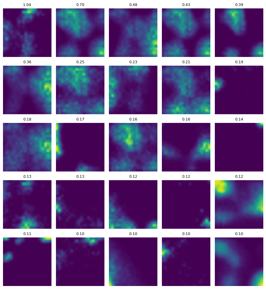
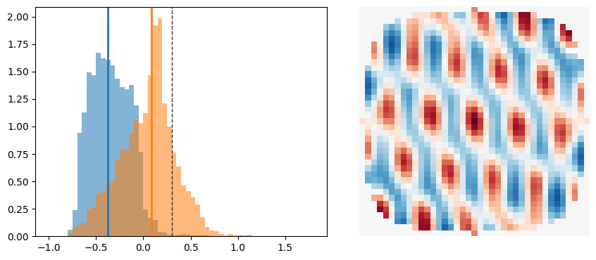
stable grid units · trained 16.6% · same weights before training 2.0%First the twin's best stable units, laid out the same way. A few can score well while showing a single blob: the score is not a perfect detector, which is why the percentages carry the result and no single map does. Then the distribution of grid scores over all active units, orange for centre-surround, blue for Gaussian, the dashed line at the cut and a solid line at each distribution's median, and beside it the autocorrelogram of one steady grid unit. In a clean lattice the peaks nearest the centre form a hexagon; at this resolution expect that pattern to show through noise, not crisply.
stable_control = np.where(control_stability > cfg["stability_min"], control_scores, -np.inf)
top_control_units = show_maps(control_maps, stable_control, cfg["units_shown"], "viridis")

fig, (ax_hist, ax_sac) = plt.subplots(1, 2, figsize=(9, 3.8))
bins = np.linspace(-1.0, 1.8, 57)
ax_hist.hist(control_scores[active_control], bins=bins, color="tab:blue", alpha=0.55, density=True)
ax_hist.hist(dog_scores[active_dog], bins=bins, color="tab:orange", alpha=0.55, density=True)
ax_hist.axvline(cut, color="0.2", ls="--", lw=1)
ax_hist.axvline(control_median_score, color="tab:blue", lw=2)
ax_hist.axvline(dog_median_score, color="tab:orange", lw=2)
# The exemplar is the steadiest grid unit that fires over a real part of the
# floor. The top scorer can be a unit with a few tiny spots, which scores well
# and draws a noisy autocorrelogram; a stable, well-covered map draws a cleaner one.
coverage = (dog_maps > 0.5 * dog_maps.max(axis=(1, 2), keepdims=True)).mean(axis=(1, 2))
candidates = np.flatnonzero(dog_grid & (coverage >= 0.15))
exemplar = (
    int(candidates[np.argmax(dog_stability[candidates])])
    if len(candidates)
    else int(top_dog_units[0])
)
ax_sac.imshow(dog_sac[exemplar].T, origin="lower", cmap="RdBu_r", vmin=-1, vmax=1)
ax_sac.axis("off")
plt.tight_layout()
plt.show()

if env.lang == "ar":
    print(
        f"وحدات سداسية مستقرة · هدف المركز والمحيط {grid_percent_dog}% · الهدف الغاوسي {grid_percent_control}%"
    )
    print(
        f"وسيط الدرجات · هدف المركز والمحيط {dog_median_score:+.2f} · الهدف الغاوسي {control_median_score:+.2f} · الفارق {median_gap:+.2f}"
    )
else:
    print(
        f"stable grid units · centre-surround {grid_percent_dog}% · Gaussian {grid_percent_control}%"
    )
    print(
        f"median score · centre-surround {dog_median_score:+.2f} · Gaussian {control_median_score:+.2f} · gap {median_gap:+.2f}"
    )
stable grid units · centre-surround 16.6% · Gaussian 0.2%
median score · centre-surround +0.09 · Gaussian -0.38 · gap +0.46
In this run 16.600% of the centre-surround network's active units were stable grid units, against 0.200% for its twin and 2% for the same weights before training. Its median grid score was 0.086, the twin's -0.377. The twin was also the better navigator, so hexagons are not what path integration needs here.
That result belongs to one seed, and the seed was chosen. A seed sets the place-cell layout, the walks and the starting weights together. Before any outcome was known, seven seeds were fixed and the centre-surround network was trained on each. All seven learned to navigate. Their shares of stable grid units were 1.0, 3.5, 4.1, 11.7, 12.8, 16.6 and 22.4%, and four of them cleared 8%. This notebook uses the 16.6% seed: the second strongest, and one whose run repeated exactly in separate sessions.
Two things held. The twin navigated more precisely in all four seeds where both networks were trained. And the centre-surround scores sat above the twin's as a whole even where the lattice barely formed: in the two weakest seeds, with grid shares close to the untrained floor, the median gap was still 0.15 and 0.19. The lean toward sixfold structure was consistent. The lattice it produces was not.
Sorscher, Mel, Ganguli and Ocko proposed the mechanism in 2019. A surround penalises both very broad and very fine spatial patterns, so the target favours units built around one preferred spatial frequency. Firing rates cannot go negative, and among single-frequency patterns under that constraint, the triangular lattice wins. That describes what the objective favours, not whether a particular training run gets there. A finite run at this scale moves toward it by an amount that depends on the seed.
Schaeffer, Khona and Fiete argued in 2022 that emergence in these models depends on choices a modeller makes and is more fragile than it first appeared, and that a network reproducing a brain's pattern is evidence about the objective, not proof that the brain is optimising it. Seven seeds here are a small instance of the same point.
One caution before leaning on the navigation gap. Position is decoded from the three most active predicted place cells, and about three quarters of the centre-surround code is a nearly flat floor, so its peak is harder to read. Part of the gap may come from a harder readout rather than worse integration, and this run cannot separate the two.
The hexagons were never asked for. The shape of the target asked for them, one step removed. It asks on every run; the lattice answers only on some.
Exercise
The network never saw a walk longer than 20 steps. Raise LENGTH_MULTIPLE and score only the steps beyond that horizon. The top row redraws the best units from before; the bottom row is the same units on long walks. The printout compares position error in centimetres inside and beyond the horizon, next to the error of always guessing the box centre. Decide which breaks first, the position readout or the lattice, and what that says about where the network keeps its sense of place.
# YOUR TURN.
# The network only ever saw walks of cfg["seq_len"] steps. Run it for longer and
# score only the steps it was never trained on. Try 1, then 3, 5, 10.
# Errors are compared in centimetres: skill is measured against standing still,
# and standing still gets worse on longer walks, which would flatter the network.
LENGTH_MULTIPLE = 5

long_len = cfg["seq_len"] * LENGTH_MULTIPLE
long_maps, _, _, long_err_cm, centre_cm = survey(
    dog_model, cfg["surround_scale"], long_len, skip=cfg["seq_len"] if LENGTH_MULTIPLE > 1 else 0
)
long_scores, _ = grid_scores(long_maps)
kept = [float(long_scores[u]) for u in top_dog_units]

fig, axes = plt.subplots(2, 8, figsize=(14, 3.8))
for i, unit in enumerate(top_dog_units[:8]):
    axes[0, i].imshow(dog_maps[unit].T, origin="lower", cmap="inferno", interpolation="gaussian")
    axes[1, i].imshow(long_maps[unit].T, origin="lower", cmap="inferno", interpolation="gaussian")
    axes[0, i].set_title(f"{dog_scores[unit]:.2f}", fontsize=9)
    axes[1, i].set_title(f"{long_scores[unit]:.2f}", fontsize=9)
for ax in axes.ravel():
    ax.axis("off")
plt.tight_layout()
plt.show()

if env.lang == "ar":
    print(
        f"مسارات أطول بـ {LENGTH_MULTIPLE} مرات · خطأ الموضع بعد أفق التدريب {long_err_cm:.1f} سم"
    )
    print(f"داخل الأفق {dog_err_cm:.1f} سم · تخمين مركز الصندوق دائماً {centre_cm:.1f} سم")
    print(
        f"متوسط درجة الوحدات نفسها {np.mean(kept):.2f} (كان {np.mean(dog_scores[top_dog_units]):.2f})"
    )
else:
    print(
        f"walks {LENGTH_MULTIPLE}× longer · position error beyond the training horizon {long_err_cm:.1f} cm"
    )
    print(
        f"within the horizon {dog_err_cm:.1f} cm · always guessing the box centre {centre_cm:.1f} cm"
    )
    print(
        f"mean score of the same units {np.mean(kept):.2f} (was {np.mean(dog_scores[top_dog_units]):.2f})"
)A hint is available in the notebook — env.hint(1)
Navigation first; the grid comparison is only meaningful if both networks passed it.
# Control first: a grid comparison between networks that cannot find their way
# would be a comparison between two kinds of noise. Then the finding that held in
# every seed measured: the centre-surround scores shifted above the twin's.
# The share of lattice units is reported, not required: across seven seeds it
# ranged from 1% to 22%, and a required check on it would fail seeds, not learners.
integrates_ok = env.check("both-integrate", min(dog_skill, control_skill))
pull_ok = env.check("surround-pull", median_gap)
grids_ok = env.check("grid-units", grid_percent_dog)✓ Path-integration skill of the weaker of the two networks: 0.484 (needs ≥ 0.35)
✓ Median grid score of the centre-surround network minus its Gaussian twin's: 0.463 (needs ≥ 0.08)
✓ Percent of centre-surround units that are grid units: above the score cut and stable across halves of the data: 16.6 (needs ≥ 8)Your completion code and the provenance of this run.
receipt = env.receipt()Workshop complete.
Completion code: AZ-██████████
Paste it on the workshop's page on Azimuth to record it.Terms in this workshop
- Recurrent Neural Network (RNN)الشبكة العصبية التكرارية
- Hidden Stateالحالة المخفية
- Path Integrationتكامل المسار
- Spatial Representationالتمثيل المكاني
- Emergent Behaviorالسلوك الناشئ
- Emergent Representationالتمثيل الناشئ
- Representation Learningتعلم التمثيلات الرقمية
- Latent Spaceالفضاء الكامن
- Neuronالعصبون الاصطناعي
- Feature Mapخريطة السمات
- Generalizationالتعميم
- Environmentالبيئة التفاعلية
- Observation Spaceفضاء المشاهدات
- Trajectoryمسار تتابع الحالات والأفعال
- Backpropagation Through Timeالتحديث التراجعي عبر الزمن