Classical MLintermediateGPU optional~30 minColab
Double Descent: Past the Interpolation Threshold
الهبوط المزدوج: ما بعد عتبة الاستيفاء
Test error peaks where parameters equal data points, not where the model gets too complex
You were taught that test error traces a U: too simple underfits, too complex overfits, and the sweet spot sits in between. So you would stop growing a model once its test error starts to climb. This workshop keeps going. It sweeps one model from a handful of parameters to twenty times more parameters than training points, and measures what the U-curve predicts and what actually happens.
The goal
Locate the test-error peak and show that it sits at the interpolation threshold, where the parameter count equals the number of training points. Confirm that the widest model fits its training data exactly, yet comes back down from the peak. Then measure why, and what removes the peak.
Colab opens a read-only copy. Save a copy to Drive to keep your edits.
The notebook needs a keyboard — best opened on a desktop.
The papers behind this
The statistics course drew one picture. On the left, a model too simple to capture the pattern: high bias, . On the right, a model so flexible it chases the noise in its training sample: high variance, . Test error is the sum of the two, so it traces a U, and the job is to stop at the bottom.
That picture is not wrong about what it describes. But it was drawn for models that stop short of fitting every training point. Modern models routinely go far past that point. The question for this workshop is simple: what happens to test error if you keep adding parameters after the training error has already reached zero?
Nothing to look for yet. This cell connects the notebook to its profile and defines the helpers that print and label figures in your language.
import azimuth_nb as azimuth

env = azimuth.setup(SLUG, lang=LANG, profile=PROFILE)


def say(en, ar_text):
    # One program, two voices: the Arabic build prints the Arabic line.
    print(ar_text if env.lang == "ar" else en)


def t(en, ar_text):
    # Figure text. matplotlib draws glyphs one by one, left to right, so raw
    # Arabic comes out as isolated letters in reversed order. Two steps fix it:
    # reshape joins the letters into their connected forms, and get_display
    # puts the line in visual order (Latin runs such as "p = n" stay readable).
    # Reshaping also drops the vowel marks, which matplotlib cannot position.
    if env.lang != "ar":
        return en
    import arabic_reshaper
    from bidi.algorithm import get_display

return get_display(arabic_reshaper.reshape(ar_text))Double Descent: Past the Interpolation Threshold
no GPU · 12.7 GB RAM · PyTorch 2.11.0+cpu
profile: free
ready · seed=17, n_train=200, n_test=2000, dim=20, noise=0.5, p_max=4000, grid_points=40, trials=5, ridge=0.01, gd_width=1000, gd_steps=20000
code · afc86a2a2abdb407To sweep model size cleanly, we need a model whose size is a single number and whose fit has no training-schedule noise. Random features give us both. The input passes through a fixed, randomly drawn layer of p ReLU units, and only the p output weights are fitted, by least squares. That makes p the parameter count. The first layer never changes, so there is no feature learning here. Whatever we find comes from the parameter count alone.
One detail matters later. When p is larger than the number of training points n, there are infinitely many weight vectors that fit the training data exactly. The solver returns the one with the smallest norm.
Note the last line: the error of a model that ignores its input and always predicts the mean. Any model worth having must beat it.
import numpy as np

cfg = env.cfg
n_train = cfg["n_train"]
n_test = cfg["n_test"]
dim = cfg["dim"]
noise = cfg["noise"]
p_max = cfg["p_max"]
trials = cfg["trials"]


def make_task(seed, n=n_train, label_noise=noise):
    # One trial = one hidden target function, one dataset, one bank of random
    # features. Every model width in a trial reuses the SAME data and the SAME
    # features (the first p columns), so the only thing that varies along the
    # sweep is the parameter count.
    rng = np.random.default_rng(seed)
    a = rng.normal(size=dim) / np.sqrt(dim)
    b = rng.normal(size=(4, dim))

    def target(x):
        # A linear part plus a few saturating bumps. Random ReLU features can
        # approximate this well, but never exactly.
        return 2.0 * (x @ a) + np.tanh(x @ b.T).sum(axis=1)

    x_tr = rng.normal(size=(n, dim))
    x_te = rng.normal(size=(n_test, dim))
    y_tr = target(x_tr) + label_noise * rng.normal(size=n)
    y_te = target(x_te)  # the test set is clean: we measure the real function
    w_feat = rng.normal(size=(p_max, dim)) / np.sqrt(dim)
    return {"x_tr": x_tr, "y_tr": y_tr, "x_te": x_te, "y_te": y_te, "w_feat": w_feat}


def features(x, w_feat, p):
    # Random ReLU features: a fixed, untrained first layer of width p.
    return np.maximum(x @ w_feat[:p].T, 0.0) / np.sqrt(p)


def fit(task, p, ridge=0.0):
    # Least squares on the first p features. With ridge = 0 and p > n there are
    # infinitely many exact fits; lstsq returns the one with the smallest norm.
    f_tr = features(task["x_tr"], task["w_feat"], p)
    f_te = features(task["x_te"], task["w_feat"], p)
    y = task["y_tr"]
    n = len(y)
    if ridge == 0.0:
        w = np.linalg.lstsq(f_tr, y, rcond=None)[0]
    elif p <= n:
        w = np.linalg.solve(f_tr.T @ f_tr + ridge * np.eye(p), f_tr.T @ y)
    else:
        w = f_tr.T @ np.linalg.solve(f_tr @ f_tr.T + ridge * np.eye(n), y)
    train_mse = float(np.mean((f_tr @ w - y) ** 2))
    test_mse = float(np.mean((f_te @ w - task["y_te"]) ** 2))
    return train_mse, test_mse, w


def width_grid(n):
    # Log-spaced widths from tiny to p_max, plus a dense band around p = n so
    # the threshold is sampled where the curve moves fastest.
    coarse = np.geomspace(5, p_max, cfg["grid_points"]).round().astype(int)
    band = np.arange(int(0.9 * n), int(1.1 * n) + 1, max(1, n // 40))
    return np.unique(np.concatenate([coarse, band, [n]]))


tasks = [make_task(cfg["seed"] + k) for k in range(trials)]
widths = width_grid(n_train)
target_var = round(float(np.mean([np.var(tk["y_te"]) for tk in tasks])), 2)

say(
    f"{trials} trials · {n_train} training points · {n_test} test points · "
    f"inputs in {dim} dimensions · label noise σ = {noise}",
    f"{trials} تجارب · {n_train} نقطة تدريب · {n_test} نقطة اختبار · "
    f"مدخلات في {dim} بُعداً · ضجيج التسميات σ = {noise}",
)
say(
    f"{len(widths)} model widths, from {widths[0]} to {widths[-1]} features",
    f"{len(widths)} عرضاً للنموذج، من {widths[0]} إلى {widths[-1]} سمة",
)
say(
    f"For scale: always predicting the mean scores a test MSE of {target_var:.2f}",
    f"للمقارنة: نموذج يتنبّأ دائماً بالمتوسط يحصل على خطأ اختبار قدره {target_var:.2f}",
)5 trials · 200 training points · 2000 test points · inputs in 20 dimensions · label noise σ = 0.5
49 model widths, from 5 to 4000 features
For scale: always predicting the mean scores a test MSE of 8.13Both axes are logarithmic. Find the classical U on the left, then watch the dashed line at p = n: what the test error does there, and what the training error does at the same moment.
import matplotlib.pyplot as plt


def sweep(ridge=0.0, n=n_train, task_list=None):
    task_list = tasks if task_list is None else task_list
    grid = width_grid(n)
    train = np.zeros((len(task_list), len(grid)))
    test = np.zeros_like(train)
    for i, tk in enumerate(task_list):
        for j, p in enumerate(grid):
            train[i, j], test[i, j], _ = fit(tk, int(p), ridge)
    # Median over trials: exactly at p = n one unlucky trial can be off by
    # orders of magnitude, and a mean would let that one trial draw the curve.
    return grid, np.median(train, axis=0), np.median(test, axis=0)


grid, train_curve, test_curve = sweep()

under = grid < n_train
best_idx = int(np.argmin(np.where(under, test_curve, np.inf)))
sweet_spot_p = int(grid[best_idx])
sweet_spot_test = round(float(test_curve[best_idx]), 2)
threshold_test = round(float(test_curve[grid == n_train][0]), 1)
widest_test = round(float(test_curve[-1]), 2)
# Captured values are rounded here, because prose quotes them verbatim.
peak_ratio = round(threshold_test / sweet_spot_test)
second_descent = round(threshold_test / widest_test)
widest_vs_sweet_spot = round(widest_test / sweet_spot_test, 2)
train_r2_widest = 1.0 - float(train_curve[-1]) / float(
    np.mean([np.var(tk["y_tr"]) for tk in tasks])
)

fig, ax = plt.subplots(figsize=(8, 4.5))
ax.plot(grid, test_curve, "o-", ms=3, label=t("test error", "خطأ الاختبار"))
# Past p = n the training error is zero to machine precision (around 1e-28).
# Drawn at its true value it would flatten everything else, so it is pinned to
# a floor: a point on the floor means "exactly fitted".
floor = 1e-2
ax.plot(
    grid,
    np.maximum(train_curve, floor),
    "s-",
    ms=3,
    alpha=0.7,
    label=t("training error", "خطأ التدريب"),
)
ax.axvline(n_train, color="grey", ls="--", lw=1)
ax.text(n_train * 1.08, floor * 2, "p = n", color="grey")
ax.scatter(
    [sweet_spot_p],
    [sweet_spot_test],
    s=80,
    facecolors="none",
    edgecolors="black",
    zorder=5,
    label=t("classical sweet spot", "النقطة المثلى الكلاسيكية"),
)
ax.set_xscale("log")
ax.set_yscale("log")
ax.set_xlabel(t("number of random features p (parameters)", "عدد السمات العشوائية p (المعاملات)"))
ax.set_ylabel(t("mean squared error (log scale)", "متوسط مربع الخطأ (مقياس لوغاريتمي)"))
ax.set_title(
    t(
        "Test error across the interpolation threshold",
        "خطأ الاختبار عبر عتبة الاستيفاء",
    )
)
ax.legend()
plt.show()

say(
    f"classical sweet spot   p = {sweet_spot_p:5d}   test MSE {sweet_spot_test:.3f}",
    f"النقطة المثلى الكلاسيكية   p = {sweet_spot_p:5d}   خطأ الاختبار {sweet_spot_test:.3f}",
)
say(
    f"interpolation threshold p = {n_train:5d}   test MSE {threshold_test:.3f}",
    f"عتبة الاستيفاء           p = {n_train:5d}   خطأ الاختبار {threshold_test:.3f}",
)
say(
    f"widest model           p = {int(grid[-1]):5d}   test MSE {widest_test:.3f}   "
    f"training MSE {train_curve[-1]:.1e}",
    f"أعرض نموذج              p = {int(grid[-1]):5d}   خطأ الاختبار {widest_test:.3f}   "
    f"خطأ التدريب {train_curve[-1]:.1e}",
)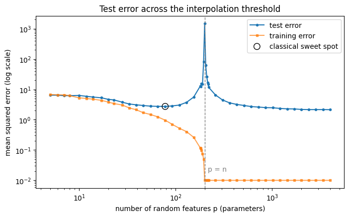
classical sweet spot   p =    78   test MSE 2.740
interpolation threshold p =   200   test MSE 1474.600
widest model           p =  4000   test MSE 2.140   training MSE 4.8e-29
Start from the left. Test error falls as features are added, because the model is underfitting and each feature helps. It bottoms out around p = 78 at a test error of 2.740, then starts to rise. Up to here, this is the curve from the course.
The rise does not level off. It turns into a spike, and the spike sits exactly at p = n = 200, the width at which the training error first reaches zero. There the test error is 1474.600: a factor of 538 above the sweet spot, and far worse than predicting the mean.
Then the curve comes back down, although the training error stays at zero all the way to 4000 features. The widest model ends at a test error of 2.140, which is 0.780 times the sweet spot's. In other words, a model that fits every noisy training label exactly ends up roughly level with the best model the classical rule would have picked.
Change the seed and that last ratio moves to either side of 1. The spike does not move: it stays at p = n, and it stays huge.
Count the options the solver has at each width. Below n, there are fewer weights than training points, so no weight vector fits every point. Least squares picks the best compromise. Above n, there are more weights than points, so infinitely many weight vectors fit every point exactly, and the solver picks the smallest.
Exactly at p = n, there is one exact fit and no choice. That single fit has to pass through every noisy label. To do it, the weights usually have to grow very large, and large weights make the model swing wildly between training points. If that account is right, the size of the weights should spike at the same place the test error does.
Compare this curve's shape with the test-error curve above. Does the spike sit at the same width?
# The size of the fitted weights, across the same sweep. Large weights mean the
# model reacts violently to small changes in its input — including the noise.
norm_curve = np.median([[np.linalg.norm(fit(tk, int(p))[2]) for p in grid] for tk in tasks], axis=0)
threshold_norm = round(float(norm_curve[grid == n_train][0]))
widest_norm = round(float(norm_curve[-1]))
sweet_spot_norm = round(float(norm_curve[best_idx]))

fig, ax = plt.subplots(figsize=(8, 3.5))
ax.plot(grid, norm_curve, "o-", ms=3, color="tab:purple")
ax.axvline(n_train, color="grey", ls="--", lw=1)
ax.set_xscale("log")
ax.set_yscale("log")
ax.set_xlabel(t("number of random features p (parameters)", "عدد السمات العشوائية p (المعاملات)"))
ax.set_ylabel(t("weight norm ‖w‖ (log scale)", "معيار الأوزان ‖w‖ (مقياس لوغاريتمي)"))
ax.set_title(
    t(
        "The fitted weights blow up exactly at p = n",
        "الأوزان المُلائَمة تنفجر عند p = n تماماً",
    )
)
plt.show()

say(
    f"weight norm at the sweet spot   p = {sweet_spot_p:5d}: {sweet_spot_norm}",
    f"معيار الأوزان عند النقطة المثلى  p = {sweet_spot_p:5d}: {sweet_spot_norm}",
)
say(
    f"weight norm at the threshold    p = {n_train:5d}: {threshold_norm}",
    f"معيار الأوزان عند العتبة         p = {n_train:5d}: {threshold_norm}",
)
say(
    f"weight norm at the widest model p = {int(grid[-1]):5d}: {widest_norm}",
    f"معيار الأوزان عند أعرض نموذج     p = {int(grid[-1]):5d}: {widest_norm}",
)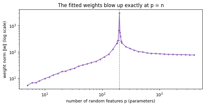
weight norm at the sweet spot   p =    78: 44
weight norm at the threshold    p =   200: 3005
weight norm at the widest model p =  4000: 77
It does. The weight norm goes from 44 at the sweet spot to 3,005 at the threshold, and falls back to 77 at the widest model. Past n, every extra feature gives the solver more ways to fit the same points, so the smallest exact fit keeps getting smaller and smoother.
This changes what "more parameters" means. In the classical picture, each parameter is more freedom to overfit. Past the threshold, each parameter is more room to fit the same data gently. Capacity alone does not decide . Which of the many exact fits you end up with decides it.
The smallest fit was the solver's choice. Here plain gradient descent, starting from zero weights, gets no instruction to keep the weights small. Look at the cosine similarity: 1 means the same direction.
# Past p = n there are infinitely many weight vectors with zero training error.
# lstsq picks the smallest one. Does ordinary gradient descent pick the same?
gd_task = tasks[0]
gd_p = cfg["gd_width"]
f_gd = features(gd_task["x_tr"], gd_task["w_feat"], gd_p)
y_gd = gd_task["y_tr"]
_, _, w_min_norm = fit(gd_task, gd_p)

w = np.zeros(gd_p)  # start at the origin, as the result depends on it
step = 1.0 / np.linalg.norm(f_gd, 2) ** 2
for _ in range(cfg["gd_steps"]):
    w -= step * f_gd.T @ (f_gd @ w - y_gd)

gd_train_mse = float(np.mean((f_gd @ w - y_gd) ** 2))
gd_cosine = round(float(w @ w_min_norm / (np.linalg.norm(w) * np.linalg.norm(w_min_norm))), 4)
say(
    f"p = {gd_p}: gradient descent reached training MSE {gd_train_mse:.1e}",
    f"عند p = {gd_p}: وصل الانحدار التدرّجي إلى خطأ تدريب {gd_train_mse:.1e}",
)
say(
    f"cosine similarity to the minimum-norm solution: {gd_cosine:.4f}",
    f"تشابه جيب التمام مع الحلّ ذي المعيار الأصغر: {gd_cosine:.4f}",
)
say(
    f"weight norms — gradient descent {np.linalg.norm(w):.1f}, "
    f"minimum norm {np.linalg.norm(w_min_norm):.1f}",
    f"معيار الأوزان — الانحدار التدرّجي {np.linalg.norm(w):.1f}، "
    f"الحلّ الأصغر {np.linalg.norm(w_min_norm):.1f}",
)p = 1000: gradient descent reached training MSE 4.6e-05
cosine similarity to the minimum-norm solution: 0.9999
weight norms — gradient descent 93.6, minimum norm 94.3Gradient descent lands on the minimum-norm fit, with a cosine similarity of 1.000. The reason is mechanical. Every gradient step is a combination of the training inputs, so starting from zero, the weights never pick up a component the data cannot see. The only exact fit with no such component is the smallest one.
So nobody had to choose the smallest fit. The optimizer chose it. This is an inductive bias: a preference built into the procedure, not written into the loss function. In deep networks the details differ, but the lesson carries over. To predict how an overparameterized model generalizes, you have to know how it was trained, not just how big it is.
Same widest model, same inputs, labels shuffled. Compare the two training errors first, then the two test errors.
# Same widest model, same inputs, but the training labels are shuffled, so
# there is no function left to learn. Can it still fit them?
shuffled = []
for k, tk in enumerate(tasks):
    rng = np.random.default_rng(cfg["seed"] + 1000 + k)
    shuffled.append(dict(tk, y_tr=rng.permutation(tk["y_tr"])))

mem = np.array([fit(tk, p_max)[:2] for tk in shuffled])
shuffled_train_mse = float(np.median(mem[:, 0]))
shuffled_test_mse = round(float(np.median(mem[:, 1])), 2)

say(
    f"p = {p_max}, true labels:     training MSE {train_curve[-1]:.1e}   test MSE {widest_test:.3f}",
    f"عند p = {p_max}، التسميات الحقيقية:  خطأ التدريب {train_curve[-1]:.1e}   خطأ الاختبار {widest_test:.3f}",
)
say(
    f"p = {p_max}, shuffled labels: training MSE {shuffled_train_mse:.1e}   test MSE {shuffled_test_mse:.3f}",
    f"عند p = {p_max}، التسميات المخلوطة:  خطأ التدريب {shuffled_train_mse:.1e}   خطأ الاختبار {shuffled_test_mse:.3f}",
)
say(
    f"predicting the mean:          test MSE {target_var:.3f}",
    f"التنبّؤ بالمتوسط:                    خطأ الاختبار {target_var:.3f}",
)p = 4000, true labels: training MSE 4.8e-29 test MSE 2.140
p = 4000, shuffled labels: training MSE 1.8e-28 test MSE 21.370
predicting the mean: test MSE 8.130Both training errors are zero. The widest model memorizes shuffled labels as perfectly as real ones. Their test errors are nothing alike: 2.140 on real labels, and 21.370 on shuffled ones, which is worse than always predicting the mean (8.130).
This is why "the model is big enough to memorize the data" cannot be the whole explanation of overfitting. The same model, at the same size, generalizes on one dataset and fails on the other. The difference lies in the data, and in how a smooth fit through it behaves between the points.
If the peak comes from forcing an exact fit through noisy labels, then allowing a slightly inexact fit should remove it. Ridge regression does that. It adds a penalty of λ times the squared weight norm, so the solver gives up a little training error to keep the weights small. The next cell reruns the same sweep, on the same data, with λ = 0.01.
The faded curve is the first sweep. The dotted line is the classical sweet spot. Look for two things: whether the peak survives, and where the best model now sits.
ridge = cfg["ridge"]
_, ridge_train_curve, ridge_test_curve = sweep(ridge=ridge)

ridge_threshold_test = round(float(ridge_test_curve[grid == n_train][0]), 2)
ridge_widest_test = round(float(ridge_test_curve[-1]), 2)
ridge_vs_sweet_spot = round(ridge_widest_test / sweet_spot_test, 2)
# How much does the regularized curve ever climb as p grows? 1.0 = never.
ridge_worst_climb = round(
    float(np.max(ridge_test_curve / np.minimum.accumulate(ridge_test_curve))), 2
)

fig, ax = plt.subplots(figsize=(8, 4.5))
ax.plot(
    grid,
    test_curve,
    "o-",
    ms=3,
    alpha=0.5,
    label=t("no penalty (minimum norm)", "بلا عقوبة (المعيار الأصغر)"),
)
ax.plot(
    grid,
    ridge_test_curve,
    "o-",
    ms=3,
    label=t(f"ridge λ = {ridge}", f"عقوبة الحافّة λ = {ridge}"),
)
ax.axhline(
    sweet_spot_test,
    color="black",
    ls=":",
    lw=1,
    label=t("classical sweet spot", "النقطة المثلى الكلاسيكية"),
)
ax.axvline(n_train, color="grey", ls="--", lw=1)
ax.set_xscale("log")
ax.set_yscale("log")
ax.set_xlabel(t("number of random features p (parameters)", "عدد السمات العشوائية p (المعاملات)"))
ax.set_ylabel(t("test MSE (log scale)", "خطأ الاختبار (مقياس لوغاريتمي)"))
ax.set_title(t("A small penalty removes the peak", "عقوبة صغيرة تُزيل القمّة"))
ax.legend()
plt.show()

say(
    f"at p = n:      no penalty {threshold_test:.3f}   ridge {ridge_threshold_test:.3f}",
    f"عند p = n:      بلا عقوبة {threshold_test:.3f}   مع الحافّة {ridge_threshold_test:.3f}",
)
say(
    f"widest model:  no penalty {widest_test:.3f}   ridge {ridge_widest_test:.3f}   "
    f"(classical sweet spot {sweet_spot_test:.3f})",
    f"أعرض نموذج:     بلا عقوبة {widest_test:.3f}   مع الحافّة {ridge_widest_test:.3f}   "
    f"(النقطة المثلى الكلاسيكية {sweet_spot_test:.3f})",
)
say(
    f"largest climb of the ridge curve above its running best: ×{ridge_worst_climb:.2f}",
    f"أكبر صعود لمنحنى الحافّة فوق أفضل قيمة سبقته: ×{ridge_worst_climb:.2f}",
)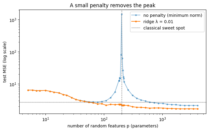
at p = n:      no penalty 1474.600   ridge 2.200
widest model:  no penalty 2.140   ridge 1.680   (classical sweet spot 2.740)
largest climb of the ridge curve above its running best: ×1.07
The peak is gone. At p = n the regularized model scores 2.200, against 1474.600 without the penalty. The curve is now close to monotone: the largest rise anywhere above its best value so far is a factor of 1.070.
The bigger change is at the right edge. The widest regularized model reaches a test error of 1.680, which is 0.610 times the classical sweet spot. The best model in the whole workshop is the largest one, with a small penalty. Unlike the unregularized ratio, this result held on every seed tried while building the workshop.
So the bias-variance tradeoff survives, but its axis was mislabelled. Variance does not grow with the parameter count. It explodes when the parameter count lands near the number of training points and the fit is forced to be exact. Move away from that point in either direction, or loosen the fit, and more parameters stop hurting.
Exercise
The next cell doubles the training set to 2n. Before you run it, set my_guess to the width where you expect the new peak. Then try halving the data instead. Here is the question to settle: is the peak's location a property of the model, or of the model and the dataset together? Then read the last line. Near the new peak, the same model does worse with more data.
# YOUR TURN.
#
# Double the training set. Before running, write down where you expect the
# peak to move — or whether it moves at all. Then try halving it.
n_new = 2 * n_train  # try n_train // 2 as well
my_guess = None  # your predicted peak location, as a width p

new_tasks = [make_task(cfg["seed"] + k, n=n_new) for k in range(trials)]
new_grid, _, new_test = sweep(n=n_new, task_list=new_tasks)
new_peak_p = int(new_grid[int(np.argmax(new_test))])
say(
    f"n = {n_new}: the test error peaks at p = {new_peak_p}"
    f" (with n = {n_train}, it peaked at p = {int(grid[int(np.argmax(test_curve))])})",
    f"عند n = {n_new}: تبلغ قمّة خطأ الاختبار p = {new_peak_p}"
    f" (وعند n = {n_train} كانت القمّة عند p = {int(grid[int(np.argmax(test_curve))])})",
)
# The same width, under the old and the new dataset size.
same_width_old = float(np.median([fit(tk, n_new)[1] for tk in tasks]))
same_width_new = float(new_test[new_grid == n_new][0])
say(
    f"a model with p = {n_new} features: test MSE {same_width_old:.2f} with "
    f"{n_train} training points, {same_width_new:.2f} with {n_new}",
    f"نموذج بـ p = {n_new} سمة: خطأ الاختبار {same_width_old:.2f} مع "
    f"{n_train} نقطة تدريب، و{same_width_new:.2f} مع {n_new}",
)
if my_guess is not None:
say(f"your guess: p = {my_guess}", f"تخمينك: p = {my_guess}")A hint is available in the notebook — env.hint(1)
The first check is the control. If the widest model did not fit its training data exactly, its low test error would just be underfitting, and the second descent would mean nothing.
# The control first: if the widest model did not actually interpolate the
# training set, the "second descent" would be an underfit model, not a
# memorizing one, and the comparison would show nothing.
interpolates_ok = env.check("widest-model-interpolates", train_r2_widest)
peak_ok = env.check("peak-at-threshold", peak_ratio)
descent_ok = env.check("second-descent", second_descent)✓ Share of training-label variance the widest model fits (R²): 1 (needs ≥ 0.999)
✓ Test error at the threshold, as a multiple of the classical sweet spot: 538 (needs ≥ 20)
✓ Test error at the threshold, as a multiple of the widest model's: 689 (needs ≥ 20)The receipt records which checks passed, the profile that ran, and the code hash.
receipt = env.receipt()Workshop complete.
Completion code: AZ-██████████
Paste it on the workshop's page on Azimuth to record it.The rule to take away is not "bigger is always better". The unregularized widest model only matched the classical sweet spot, and the seed decided which side of it it landed on. The corrected rule is narrower and more useful. Test error peaks where the parameter count meets the dataset size and the fit is forced to be exact. Past that point, the optimizer's preference for small, smooth solutions takes over. With a little regularization, the largest model is the best one.
Terms in this workshop
- Generalizationالتعميم
- Overfittingفرط التخصيص
- Underfittingضعف مواءمة البيانات (التعلم الناقص)
- Optimizationالأمثَلَة
- Memorizationالحفظ