Neural NetworksintermediateGPU optional~30 minColab
Anomaly detection with an autoencoder
كشف الشذوذ بالمُرمِّز الذاتي
Reconstruction error as a distance
You have 5,000 heartbeat recordings and almost no labels for the abnormal ones, because abnormal is exactly what nobody collected enough of. This is the ordinary shape of : the rare class is rare in your training data too, so a classifier has nothing to learn from. Train a model on normal alone, and let its failure to reconstruct the unfamiliar be the signal.
The goal
Train an autoencoder on normal heartbeats only, choose a threshold from the reconstruction-error distribution rather than by guessing, and reach at least 0.90 F1 on a held-out set that contains both classes.
Colab opens a read-only copy. Save a copy to Drive to keep your edits.
The notebook needs a keyboard — best opened on a desktop.
The papers behind this
A classifier needs examples of every class it will meet. Anomaly detection is the case where you cannot have them: the interesting class is rare by definition, and the examples you do have are not representative of the ones you have not seen yet. So we invert the problem. Train a model to do something easy — copy its input to its output — but force it through a layer too narrow to copy everything. It will spend that budget on whatever is common. Then feed it something uncommon, and watch it fail.
Preflight: the runtime is checked and the dataset verified before anything trains.
import azimuth_nb as azimuth

env = azimuth.setup(SLUG, lang=LANG, profile=PROFILE)Anomaly detection with an autoencoder
no GPU · 3.9 GB RAM · PyTorch 2.2.2+cu121
profile: free
assets:
· ecg5000.csv — already present
ready · epochs=160, batchSize=128, latentDim=8, hidden=[64, 32], learningRate=0.001, seed=17Note the split: the training set is normal traces only. That is the whole method.
import numpy as np

raw = np.loadtxt(env.assets["ecg5000.csv"], delimiter=",")
traces, labels = raw[:, :-1].astype(np.float32), raw[:, -1].astype(int)

# Min-max to [0, 1] using TRAINING statistics only. Fitting the scaler on
# everything would leak the abnormal range into the normal model — a quiet
# mistake that inflates every number downstream.
rng = np.random.default_rng(env.cfg["seed"])
order = rng.permutation(len(traces))
traces, labels = traces[order], labels[order]

split = int(0.8 * len(traces))
train_all, test_x = traces[:split], traces[split:]
train_labels, test_y = labels[:split], labels[split:]

# THE METHOD, IN ONE LINE: the model only ever sees normal traces.
train_x = train_all[train_labels == 1]

lo, hi = train_x.min(), train_x.max()
train_x = (train_x - lo) / (hi - lo)
test_x = (test_x - lo) / (hi - lo)

n_normal = int((test_y == 1).sum())
n_abnormal = int((test_y == 0).sum())
class_balance = {
    "trainNormal": len(train_x),
    "testNormal": n_normal,
    "testAbnormal": n_abnormal,
}

if env.lang == "ar":
    print(f"التدريب: {len(train_x)} أثراً طبيعياً فقط")
    print(f"الاختبار: {n_normal} طبيعي · {n_abnormal} شاذ")
else:
    print(f"train: {len(train_x)} normal traces only")
print(f"test: {n_normal} normal · {n_abnormal} abnormal")train: 2338 normal traces only
test: 581 normal · 419 abnormalimport torch
import torch.nn as nn
torch.manual_seed(env.cfg["seed"])
device = torch.device("cuda" if torch.cuda.is_available() else "cpu")
n_features = train_x.shape[1]
class Autoencoder(nn.Module):
"""Symmetric encoder/decoder around a deliberately narrow layer.
The bottleneck width is the entire experiment. Widen it and the model
learns the identity function and reconstructs abnormal traces just as well
as normal ones — at which point there is no detector left, only a copier.
"""
def __init__(self, n_features: int, hidden: list[int], latent: int):
super().__init__()
widths = [n_features, *hidden]
encoder: list[nn.Module] = []
for a, b in zip(widths[:-1], widths[1:]):
encoder += [nn.Linear(a, b), nn.ReLU()]
encoder += [nn.Linear(widths[-1], latent), nn.ReLU()]
self.encoder = nn.Sequential(*encoder)
decoder: list[nn.Module] = []
rev = [latent, *hidden[::-1]]
for a, b in zip(rev[:-1], rev[1:]):
decoder += [nn.Linear(a, b), nn.ReLU()]
# Sigmoid because the inputs were scaled to [0, 1]: the output range
# should be able to reach the input range and no further.
decoder += [nn.Linear(rev[-1], n_features), nn.Sigmoid()]
self.decoder = nn.Sequential(*decoder)
def forward(self, x):
return self.decoder(self.encoder(x))
model = Autoencoder(n_features, list(env.cfg["hidden"]), env.cfg["latentDim"]).to(device)
param_count = sum(p.numel() for p in model.parameters())
env.explain("bottleneck")
if env.lang == "ar":
print(f"عنق الزجاجة: {env.cfg['latentDim']} من أصل {n_features} بُعداً · {param_count:,} معامل")
else:
print(f"bottleneck: {env.cfg['latentDim']} of {n_features} dims · {param_count:,} parameters")bottleneck — The narrowest layer of an autoencoder. Its width is the budget: the model must describe the whole input in this many numbers.
bottleneck: 8 of 140 dims · 22,868 parametersWatch the shape, not just the last number. The loss drops hard, then sits on a plateau for twenty or thirty epochs, then breaks downward again — the model has stopped improving the average trace and started fitting the parts it had been averaging over. Stop it on the plateau and you ship a half-trained detector that looks converged.
from torch.utils.data import DataLoader, TensorDataset

train_t = torch.from_numpy(train_x).to(device)
loader = DataLoader(
    TensorDataset(train_t, train_t),
    batch_size=env.cfg["batchSize"],
    shuffle=True,
)

optimizer = torch.optim.Adam(model.parameters(), lr=env.cfg["learningRate"])
criterion = nn.MSELoss()

loss_curve = []
model.train()
for epoch in range(env.cfg["epochs"]):
    total = 0.0
    for batch_x, batch_y in loader:
        optimizer.zero_grad()
        loss = criterion(model(batch_x), batch_y)
        loss.backward()
        optimizer.step()
        total += loss.item() * len(batch_x)
    epoch_loss = total / len(train_t)
    loss_curve.append(epoch_loss)
    if epoch % 10 == 0 or epoch == env.cfg["epochs"] - 1:
        print(f"epoch {epoch:3d}  loss {epoch_loss:.5f}")

final_loss = loss_curve[-1]epoch 0 loss 0.02346
epoch 10 loss 0.00169
epoch 20 loss 0.00169
epoch 30 loss 0.00168
epoch 40 loss 0.00166
epoch 50 loss 0.00160
epoch 60 loss 0.00123
epoch 70 loss 0.00114
epoch 80 loss 0.00093
epoch 90 loss 0.00075
epoch 100 loss 0.00071
epoch 110 loss 0.00070
epoch 120 loss 0.00068
epoch 130 loss 0.00066
epoch 140 loss 0.00062
epoch 150 loss 0.00058
epoch 159 loss 0.00057The picture the whole workshop is for: two distributions, and the gap between them.
import matplotlib.pyplot as plt


def reconstruction_error(x: np.ndarray) -> np.ndarray:
    """Mean absolute error per trace — one number for each recording.

    L1 rather than L2 on purpose: squared error lets a single badly-missed
    sample dominate a trace's score, which makes the threshold sensitive to
    noise rather than to shape.
    """
    model.eval()
    with torch.no_grad():
        t = torch.from_numpy(x).to(device)
        return torch.mean(torch.abs(model(t) - t), dim=1).cpu().numpy()


train_errors = reconstruction_error(train_x)
test_errors = reconstruction_error(test_x)

normal_errors = test_errors[test_y == 1]
abnormal_errors = test_errors[test_y == 0]
separation = float(abnormal_errors.mean() / normal_errors.mean())

env.explain("reconstruction error")
fig, ax = plt.subplots(figsize=(7, 3.6))
bins = np.linspace(0, float(np.percentile(test_errors, 99.5)), 60)
ax.hist(normal_errors, bins=bins, alpha=0.75, label="normal", color="#2a9d8f")
ax.hist(abnormal_errors, bins=bins, alpha=0.75, label="abnormal", color="#e76f51")
ax.set_xlabel("reconstruction error (MAE)")
ax.set_ylabel("traces")
ax.legend()
ax.spines[["top", "right"]].set_visible(False)
fig.tight_layout()
plt.show()

print(f"normal mean   {normal_errors.mean():.4f}")
print(f"abnormal mean {abnormal_errors.mean():.4f}")
separation_ok = env.check("separation", separation)reconstruction error — How far the output is from the input. On data the model was trained on it is small; on unfamiliar data it is not, and that gap is the detector.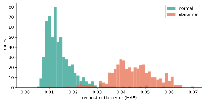
normal mean   0.0146
abnormal mean 0.0452
✓ Abnormal error, as a multiple of normal error: 3.103 (needs ≥ 2.5)
Exercise
Choose the . The obvious move is to try values until F1 peaks — but that uses the abnormal labels, which you would not have on the day you deploy. Use the training errors instead: pick a percentile of the errors on data the model has already seen, and justify the number you picked.
Then look at what the numbers above are telling you. Training this model for 1160 epochs instead of 60 pushed the separation from 2.5× to 3.1× — the two distributions moved measurably further apart — and F1 did not move at all, because rose by as much as fell. The detector is no longer limited by the model. It is limited by this cell. Find a threshold that beats 0.949, and notice that you did it without retraining anything.
# YOUR TURN.
#
# Pick a percentile of `train_errors` — the errors on traces the model was
# trained on. Anything you can compute from this array is available on the day
# you deploy, with no abnormal examples in hand. Anything you compute from
# `abnormal_errors` is not.
#
# Start here and change the number, with a reason:
PERCENTILE = 95

threshold = float(np.percentile(train_errors, PERCENTILE))
print(f"threshold = {threshold:.4f} (p{PERCENTILE} of training error)")A hint is available in the notebook — env.hint(2)
predicted_abnormal = test_errors > threshold
actually_abnormal = test_y == 0

tp = int((predicted_abnormal & actually_abnormal).sum())
fp = int((predicted_abnormal & ~actually_abnormal).sum())
fn = int((~predicted_abnormal & actually_abnormal).sum())
tn = int((~predicted_abnormal & ~actually_abnormal).sum())

precision = tp / (tp + fp) if (tp + fp) else 0.0
recall = tp / (tp + fn) if (tp + fn) else 0.0
f1 = 2 * precision * recall / (precision + recall) if (precision + recall) else 0.0
confusion = {"tp": tp, "fp": fp, "fn": fn, "tn": tn}

if env.lang == "ar":
    print(f"الدقة {precision:.3f} · الاستدعاء {recall:.3f} · F1 {f1:.3f}")
    print(f"أخطأ في {fn} حالة شاذة، وأنذر زوراً في {fp} حالة طبيعية")
else:
    print(f"precision {precision:.3f} · recall {recall:.3f} · F1 {f1:.3f}")
    print(f"missed {fn} abnormal · false-alarmed on {fp} normal")

f1_ok = env.check("f1", f1)precision 0.925 · recall 0.969 · F1 0.946
missed 13 abnormal · false-alarmed on 33 normal
✓ F1 on the held-out set: 0.9464 (needs ≥ 0.9)Isolation Forest reaches 0.780 against the autoencoder's 0.946. The comparison is the point, not the win — read which one you would actually ship.
from sklearn.ensemble import IsolationForest

forest = IsolationForest(
    n_estimators=100,
    contamination=n_abnormal / len(test_y),
    random_state=env.cfg["seed"],
)
forest.fit(train_x)
forest_abnormal = forest.predict(test_x) == -1

b_tp = int((forest_abnormal & actually_abnormal).sum())
b_fp = int((forest_abnormal & ~actually_abnormal).sum())
b_fn = int((~forest_abnormal & actually_abnormal).sum())
b_precision = b_tp / (b_tp + b_fp) if (b_tp + b_fp) else 0.0
b_recall = b_tp / (b_tp + b_fn) if (b_tp + b_fn) else 0.0
baseline_f1 = (
    2 * b_precision * b_recall / (b_precision + b_recall) if (b_precision + b_recall) else 0.0
)

print(f"isolation forest F1 {baseline_f1:.3f} · autoencoder F1 {f1:.3f}")isolation forest F1 0.780 · autoencoder F1 0.946The receipt: your completion code, and the numbers it was derived from.
receipt = env.receipt()Workshop complete.
Completion code: AZ-██████████
Paste it on the workshop's page on Azimuth to record it.Terms in this workshop
- Bottleneckعنق الزجاجة
- Reconstruction Errorخطأ إعادة البناء
- Thresholdالعتبة
- Latent Spaceالفضاء الكامن